By
By
What is Feature Engineering?
Feature Engineering in machine learning is creating new features from existing data. Often, with raw data, the information contained within may not be sufficient from a learning perspective. Because of this, you may need to transform this data into new features or columns that help you represent the data in a way that is more useful for learning. The general process of building a model is as follows.
- Exploratory Data Analysis including Data Cleaning
- Feature Engineering (This article)
- Feature Selection
- Model Selection
- Model Training and Evaluation
Of all these steps, arguably the most important is the Feature Engineering step. By defaulting only to the raw data, you risk missing out on providing valuable context as to why a behavior is happening. Whether predicting the behavior of a user, or a machine, Feature Engineering is crucial to the success of your project. A few examples of what might need to be done:
- Scaling numeric data and encoding categorical data
- Converting long-form text into a numerical values
- Calculate the difference between dates or times
- Aggregate data into a single row, such as summing, counting, or calculating averages
- Creating aggregate date windows
- Merge data from different sources into a single set of observations
I liked the definition provided on Wikipedia. It sums up the idea of using domain knowledge to extract new features:
Feature engineering or feature extraction is the process of using domain knowledge to extract features (characteristics, properties, attributes) from raw data. The motivation is to use these extra features to improve the quality of results from a machine learning process, compared with supplying only the raw data to the machine learning process.
We can start with just that; domain knowledge.
Domain Knowledge
One of the critical parts of feature engineering is applying business and domain knowledge to your data to create the best features. There is not a single way or rule on how to create features, but many of the methods require you to know the context of why they might be relevant.
For this example, the dataset we'll use was synthetically generated (by the Author) to represent companies that have purchased software and randomly generated usage data to simulate events that a user might attempt in their day-to-day use of the software.
When brainstorming what features you might want to create, think about the context of the data. We will create several features that represent how active an account is for this. We will demonstrate a number of these below.
First, we need to understand how the data is structured and the relationships.
Understanding Our Data Structure
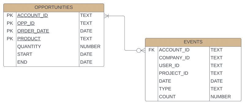
Let's look at this visualized with an Entity Relationship Diagram or ERD. An ERDs is the best way to visualize tables of information. We can see everything we need to and how the data from columns, types, and relationships in a single image.
In our first table, OPPORTUNITIES, we have a composite key that makes up the primary key consisting of ACCOUNT_ID, OPPORTUNITY_ID, RENEWAL_DATE, and PRODUCT_CODE. The primary key allows us to identify an opportunity uniquely. In the EVENTS table, we have a foreign key relationship with ACCOUNT_ID. For each account, we have zero to many potential events.
Now that we have a general understanding of the data structure, we can import our data and start the process of Feature Engineering.
Loading and Cleaning the Data
The first step is to load and clean our data. We can understand here the size and shape of our data as well.
import pandas as pd

df_opp = pd.read_csv('opps.csv')
df_event = pd.read_csv('events.csv')
print(df_opp.shape)
print(df_event.shape)
(1000, 8)
(1048575, 7)
We see that we have about 1,000 opportunities and 1,000,000 events.
df_opp.info()
<class 'pandas.core.frame.DataFrame'>
RangeIndex: 1000 entries, 0 to 999
Data columns (total 7 columns):
 #   Column      Non-Null Count  Dtype
---  ------      --------------  -----
 0   ACCOUNT_ID  1000 non-null   object
 1   OPP_ID      1000 non-null   object
 2   ORDER_DATE  1000 non-null   object
 3   PRODUCT     1000 non-null   object
 4   QUANTITY    1000 non-null   int64
 5   START       998 non-null    object
 6   END         998 non-null    object
dtypes: int64(1), object(6)
memory usage: 54.8+ KB
df_event.info()
<class 'pandas.core.frame.DataFrame'>
RangeIndex: 1048575 entries, 0 to 1048574
Data columns (total 7 columns):
 #   Column      Non-Null Count    Dtype
---  ------      --------------    -----
 0   ACCOUNT_ID  1048575 non-null  object
 1   COMPANY_ID  1048575 non-null  object
 2   USER_ID     1048575 non-null  object
 3   PROJECT_ID  977461 non-null   object
 4   DATE        1048575 non-null  object
 5   TYPE        1048575 non-null  object
 6   COUNT       1048575 non-null  int64
dtypes: int64(1), object(6)
memory usage: 56.0+ MB
Both tables contain mostly strings (objects) with one numeric column.
df_event.head()
   ACCOUNT_ID COMPANY_ID USER_ID PROJECT_ID       DATE  \
0  account420       org1      u1         p1 2019-05-10
1  account399       org2      u2         p2 2019-05-06
2  account399       org2      u3         p3 2019-06-24
3  account122       org3      u4         p4 2019-04-30
4   account61       org4      u5         p5 2019-08-07

                                                TYPE  COUNT
0  099664351c56c479154c4b1e649a727e3ac099cc26747c...      3
1  78478722fa50547376912d1bc1b21d5f5fb60188015342...      1
2  9e5fd45ed38136db73e76b46ad11a0200b7a4cbaae9bc1...      2
3  85c11686c1e1d3072f30b05ff74fd93b92c5d37a1b7ba3...      1
4  31ea88da80c3371a7e70ac8a9299974290c47e83b46170...      1
df_opp.head()
  ACCOUNT_ID OPP_ID ORDER_DATE  \
0   account1   opp1 2020-04-23
1   account1   opp1 2020-04-23
2   account2   opp2 2020-04-16
3   account2   opp2 2020-04-16
4   account3   opp3 2020-04-09

                                             PRODUCT  QUANTITY
0  cd5ba48bb6ce3541492df6f2282ca555a65397c168dc59...         4
1  1a5a6aac31b1d9e08401bd147df106c600254b2df05a3f...         2
2  28746a25d12d36a1c0956436cfd6959f0db252e3020928...         1
3  1a5a6aac31b1d9e08401bd147df106c600254b2df05a3f...         8
4  1a5a6aac31b1d9e08401bd147df106c600254b2df05a3f...         3

  START         END
0 2020-04-24    2021-04-23
1 2020-04-24    2021-04-23
2 2020-04-17    2021-04-16
3 2020-04-17    2021-04-16
4 2020-04-10    2021-04-09
A typical part of this process is to ensure that we do not have null values. After inspection of the data (not shown), we have a few things. We have some null values in our OPPtable, we'll drop these for simplicity, and with the EVENTS table, we have a few null values for the PROJECT_ID, which we can fill with another value, such as the COMPANY_ID. It takes understanding the business context of handling null values; these are just two examples.
# Drop any null values from important variables
df_opp.dropna(inplace=True)

# Fill any missing PROJECT_IDS with the COMPANY_ID
df_event['PROJECT_ID'].fillna(df_event['COMPANY_ID'], inplace=True)
Scaling Numeric Data and Encoding Categorical Data
A very simple transformation of data is scaling numerical data and encoding categorical data. While numeric scaling of data isn't feature engineering, it is important since many algorithms do not like data that isn't scaled.
A common method for transforming categorical data is to use a process known as One-Hot-Encoding or OHE. OHE takes categorical data and expands them into new columns where there is a new column for each categorical value and a binary value indicating if that category is in the row or not. OHE prevents models from predicting values between ordinal values. For more information on OHE, check out: One Hot Encoding.
A typical process for this is to wrap and utilize a column transformer. You can read more about this process here: Stop Building Your Models One Step at a Time. Automate the Process with Pipelines!
column_trans = ColumnTransformer(transformers=
        [('num', MinMaxScaler(), selector(dtype_exclude="object")),
        ('cat', OneHotEncoder(), selector(dtype_include="object"))],
        remainder='drop')
Converting Long-Form Text into a Numeric Values
Another common method for dealing with long text data is to represent the length of the text as a number, useful in cases such as product reviews. For example, are long reviews typically tied to more negative or positive reviews? Are longer reviews more useful, so the product associated with them tends to sell better? You might need to experiment with this. Our dataset doesn't have long-form text, but here is an example of how to do this.
df['text_len'] = df.apply(lambda row: len(row['text']), axis = 1)
Calculate the Difference Between Dates or Times
Typically, a date itself is not a useful feature in machine learning. What does 01/05/2021 mean versus 05/01/2012? We need to convert these into something more useful for learning. Or example, we are talking about sales opportunities whether or not a customer will continue to purchase or subscribe to our theoretical product. Something that might be more useful is to capture if the customer has been active recently. A customer that has not been active would most likely not re-purchase our software.
First, you need to ensure that any dates are actually in a date-time format. To accomplish this, we can utilize Pandas to_datetime function.
# Convert dates to datetime type
df_event['DATE'] = pd.to_datetime(df_event['DATE'])
df_opp['ORDER_DATE'] = pd.to_datetime(df_opp['ORDER_DATE'])
df_opp['START'] = pd.to_datetime(df_opp['START'])
df_opp['END'] = pd.to_datetime(df_opp['END'])
Next, we can construct new columns that represent the number of days since the last time they utilized the software. After we have converted to the date-time format, it's a simple subtraction operation and storing it as a new column called DAYS_LAST_USED.
Note: This calculation is done last in our notebook but fits better with the article.
# Add a column for the number of days transpired since the last known event and the renewal datedf['DAYS_LAST_USED'] = (df['ORDER_DATE'] - df['DATE']).dt.days
Aggregate Data Into a Single Row Such as Summing, Counting, or Calculating Averages
A critical step is making sure we only have one row or one observation that represents each unique opportunity. As We saw above during import as having 1,000 customers but 1,000,000 events. We need to aggregate our events into a single row for each account or opportunity. For our example, we will aggregate events by the ACCOUNT_ID.
Pandas has an amazing feature for this with groupby called .agg. We can aggregate all the columns with different aggregate operators in a single operation. Here you can pass a function name string like sum or count. You can utilize Numpy functions like mean and std or even pass a custom function; it's incredibly powerful. Read more In the Pandas Documentation.
Take note of nunique - a powerful way to count the number of unique values in a column. Very powerful for categorical data.
df_agg = df_event.groupby(['ACCOUNT_ID'], as_index=False).agg(
    {
        # how many unique projects are they using (more is better)
        'PROJECT_ID':"nunique",

        # how many different unique orgs (more is better)
        'COMPANY_ID':"nunique",

        # how many total unique users (more is better)
        'USER_ID':'nunique',

        # are the using the software recently (more recent is better)
        'DATE':max,

        # how many different features are they using (more is better)
        'TYPE':"nunique",

        # what is their utilization (larger is better)
        'COUNT':sum
    }
)

df_agg.head()
   ACCOUNT_ID  PROJECT_ID  COMPANY_ID  USER_ID       DATE  TYPE  COUNT
0    account1           6           1        6 2019-09-23    21    216
1   account10         116           1       19 2019-10-23   309  87814
2  account100           9           1        5 2019-10-29   188   1582
3  account101           3           1        1 2019-09-18    31    158
4  account102          35           1        3 2019-10-30   214  14744
After the aggregation is complete, we now have a simple Data Frame with a numeric representation for each column, including the maximum date the product was last utilized, which can then be used to convert it to a numeric value as shown above.
Creating Aggregate Date Windows
Another excellent Feature Engineering technique is to create different aggregate counts based on rolling timeframes. For example, how active was a customer over the past week, month, or quarter? Similar to the idea with the number of days since the account was last active, we calculated the amount of usage during these time windows. Certainly, more active users, more recently, will most likely imply the desire to keep utilizing the software.
Pandas have incredible functionality for working with Time Series data. You can read more about it the Pandas Documentation. One of the caveats to working with Time Series functions is that you need a date-time-based index. So the first thing we will do is set the index to our DATEcolumn.
# in order to use "last" calculations, you need a date based index
df_ts = df_event.set_index('DATE')
Next, we can use an operation that allows us to aggregate by the last number of days (weeks, months, years) and utilize a groupby operation and aggregator such as sum like we did above. Because we want to store a few of these values, we'll first calculate them, save them as a new Data Frame, and rename the column to something more descriptive.
df_14 = df_ts.last('14D').groupby('ACCOUNT_ID')[['COUNT']].sum()
df_14.rename(columns={"COUNT": "COUNT_LAST_14"}, inplace=True)

df_30 = df_ts.last('30D').groupby('ACCOUNT_ID')[['COUNT']].sum()
df_30.rename(columns={"COUNT": "COUNT_LAST_30"}, inplace=True)

df_60 = df_ts.last('60D').groupby('ACCOUNT_ID')[['COUNT']].sum()
df_60.rename(columns={"COUNT": "COUNT_LAST_60"}, inplace=True)
Finally, we'll merge these back into our main aggregated Data Frame, appending our three new features.
df_agg = pd.merge(df_agg, df_14, on="ACCOUNT_ID", how='left')
df_agg = pd.merge(df_agg, df_30, on="ACCOUNT_ID", how='left')
df_agg = pd.merge(df_agg, df_60, on="ACCOUNT_ID", how='left')

# Finally - fill null values with Zeros for future modeling
df_agg.fillna(0, inplace=True)
df_agg.sample(10)
     COUNT_LAST_14  COUNT_LAST_30  COUNT_LAST_60
340        12107.0        46918.0          87659
472           88.0         1502.0           2042
295           47.0          262.0            412
453          955.0         5921.0          13915
242          175.0          663.0            946
286          165.0         1106.0           2066
461          469.0         3722.0           7984
85           503.0         1954.0           4183
46           157.0         1808.0           3165
444            0.0            2.0              2
Merge Data From Different Sources Into a Single set of Observations
Finally, we need to merge our newly aggregated EVENTS table with all of our features into the OPPS Data Frame. We can do this with the same merge function above.
# Merge the datasets on Account ID
df = pd.merge(df_opp, df_agg, on="ACCOUNT_ID")
df
  ACCOUNT_ID OPP_ID ORDER_DATE  \
0   account1   opp1 2020-04-23
1   account1   opp1 2020-04-23
2   account2   opp2 2020-04-16
3   account2   opp2 2020-04-16
4   account3   opp3 2020-04-09

                                  PRODUCT    QUANTITY      START
0  cd5ba48bb6ce3541492df6f2282ca555a65...           4 2020-04-24
1  1a5a6aac31b1d9e08401bd147df106c6002...           2 2020-04-24
2  28746a25d12d36a1c0956436cfd6959f0db...           1 2020-04-17
3  1a5a6aac31b1d9e08401bd147df106c6002...           8 2020-04-17
4  1a5a6aac31b1d9e08401bd147df106c6002...           3 2020-04-10

         END  PROJECT_ID       DATE  DAYS_LAST_USED  TYPE  COUNT
0 2021-04-23           6 2019-09-23             213    21    216
1 2021-04-23           6 2019-09-23             213    21    216
2 2021-04-16          22 2019-10-16             183   185  19377
3 2021-04-16          22 2019-10-16             183   185  19377
4 2021-04-09          27 2019-10-08             184    64    556

   COUNT_LAST_14  COUNT_LAST_30  COUNT_LAST_60  DAYS_LAST_USED
0            7.0          136.0            216             213
1            7.0          136.0            216             213
2         1157.0        10109.0          19314             183
3         1157.0        10109.0          19314             183
4            7.0          372.0            556             184
df.shape
(949, 13)
And there you have it! In our final Data Frame, we have about 1,000 rows (after dropping null values) with our newly created features appended. Based on these new features, we can perform Feature Selection and train the model.
For the full code for this article, please visit GitHub
Conclusion
Feature Engineering is arguably the most critical step in Machine Learning. Feature Engineering is creating new columns in your data by using domain and business knowledge to construct new information from the data. We covered multiple techniques for dealing with categorical data, multiple methods for working with date-time data, and how to aggregate multiple observations into new representations that can be merged back into the original data. While this scratches the topic's surface, I hope it gets you started on your journey!