By
By
What is Feature Selection?
Feature Selection in Machine Learning is selecting the most impactful features, or columns, in a dataset. Does your dataset have many columns, and do you want to see which have the biggest impact? Do you want to discard those that aren't generating much value? By performing feature selection, you're not only reducing the amount of datathat needs to be processed to speed up your analysis, but you're simplifying the interpretation of the model, making it easier to understand.
Depending on the types of data you have, one can use several techniques, ranging from Statistical methods to leveraging a machine learning model to make the selection. We'll look at a few of the most common techniques and see how they are applied in practice!
- Categorical data using the Chi-Squared Test
- Pearson's Correlation Coefficient for Numeric Data
- Principal Component Analysis for Numeric Data
- Feature Importance with Random Forests for Both Categorical and Numeric Data
Let's get started!
Data and Imports
For our demonstration today, we will use the Bank Marketing UCI dataset, which one can find on Kaggle. This dataset contains information about Bank customers in a marketing campaign, and it contains a target variable that one can utilize in a classification model. This dataset is in the public domain under CC0: Public Domain and can be used.
For more information on building classification models, check out: Everything You Need to Know to Build an Amazing Binary Classifier and Go Beyond Binary Classification with Multiclass and Multi-Label Models
We will start by importing the necessary libraries and loading the data. We'll be utilizing Scikit-Learn for each of our different techniques. In addition to what is demonstrated here, there are many other supported methods.
import pandas as pd

from sklearn.model_selection import train_test_split
from sklearn.feature_selection import chi2
from sklearn.feature_selection import SelectKBest
from sklearn.preprocessing import LabelEncoder, OrdinalEncoder
from sklearn.ensemble import RandomForestClassifier
from sklearn.preprocessing import MinMaxScaler
from sklearn.compose import ColumnTransformer
from sklearn.preprocessing import LabelEncoder
from sklearn.compose import make_column_selector as selector
from sklearn.pipeline import Pipeline

import matplotlib.pyplot as plt
import seaborn as sns

df = pd.read_csv("bank.csv", delimiter=";")
Feature Selection for Categorical Values
If your dataset is all categorical in nature, we can use the Pearson's Chi-Squared Test. According to Wikipedia:
The Chi-Squared test is a statistical test applied to categorical data to evaluate how likely it is that any observed difference between the sets arose by chance.
You apply the Chi-Squared test when both your feature data is categorical as well as your target data is categorical e.g., classification problems.
Note: While this dataset contains a mix of categorical and numeric values, we'll isolate the categorical values to demonstrate how you would apply the Chi-Squared test. A better method for this dataset will be described below via Feature Importances to select features across categorical and numeric types.
We'll start by selecting only those types that are categorical or of type object in Pandas. Pandas stores text as objects, so you should validate if these are absolute values before simply utilizing the object type.
# get categorical data
cat_data = df.select_dtypes(include=['object'])
We can then isolate the features and the target values. The target variable, y is the last column in the Data Frame and therefore we can use Python's slicing technique to separate them into X and y.
X = cat_data.iloc[:, :-1].values
y = cat_data.iloc[:,-1].values
Next we have two functions. These functions will use the OrdinalEncoder for the X data and the LabelEncoder for the y data. As the name implies, the OrdinalEncoder will convert categorical values to numerical representation honoring a specific order. By default the encoder automatically selects this order, however, you can provide a list of values for an order if desired. The LabelEncoder will convert like values into numerical representations. Per Scikit-Learn's documentation, you should only use the LabelEncoder on the target variable.
def prepare_inputs(X_train, X_test):
    oe = OrdinalEncoder()
    oe.fit(X_train)
    X_train_enc = oe.transform(X_train)
    X_test_enc = oe.transform(X_test)
    return X_train_enc, X_test_enc

def prepare_targets(y_train, y_test):
    le = LabelEncoder()
    le.fit(y_train)
    y_train_enc = le.transform(y_train)
    y_test_enc = le.transform(y_test)
    return y_train_enc, y_test_enc
Next, we'll split our data into train and test sets and process the data with the above functions. Note how the above functions fit the encoders only to the training data and then transform both train and test data.
X_train, X_test, y_train, y_test = train_test_split(X,
                                                    y,
                                                    test_size=0.33,
                                                    random_state=1)
# prepare input data
X_train_enc, X_test_enc = prepare_inputs(X_train, X_test)
# prepare output data
y_train_enc, y_test_enc = prepare_targets(y_train, y_test)
Next is a function that will help us select the best features utilizing the Chi-Squared test inside the SelectKBest method. We can start by setting the argument k='all', which will first run the test across all features, and later we can apply it with a specific number of features.
def select_features(X_train, y_train, X_test, k_value='all'):
    fs = SelectKBest(score_func=chi2, k=k_value)
    fs.fit(X_train, y_train)
    X_train_fs = fs.transform(X_train)
    X_test_fs = fs.transform(X_test)
    return X_train_fs, X_test_fs, fs
We can start by printing off the scores for each feature.
# feature selection
X_train_fs, X_test_fs, fs = select_features(X_train_enc,
                                            y_train_enc,
# what are scores for the features
names = []
values = []
for i in range(len(fs.scores_)):
    names.append(cat_data.columns[i])
    values.append(fs.scores_[i])
chi_list = zip(names, values)

# plot the scores
plt.figure(figsize=(10,4))
sns.barplot(x=names, y=values)
plt.xticks(rotation = 90)
plt.show()
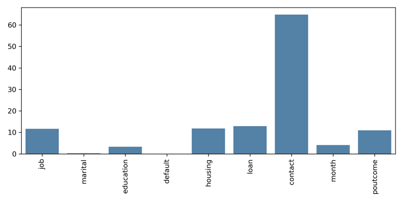
Here, we see that contact has the largest score while marital, default, and month have the lowest. Overall it looks like there are about 5 features that are worth considering. We'll use the SelectKBest method to select the top 5 features.
X_train_fs, X_test_fs, fs = select_features(X_train_enc, y_train_enc, X_test_enc, 5)
And we can print the top features, the values corresponding to their index above.
fs.get_feature_names_out()
array(['x0', 'x4', 'x5', 'x6', 'x8'], dtype=object)
And finally, we can print the shape of the X_train_fs and X_test_fs data and see that the second dimension is 5 for the selected features.
print(X_train_fs.shape)
print(X_test_fs.shape)
(3029, 5)
(1492, 5)
Feature Selection for Numeric Values
When dealing with pure numeric data, there are two methods that I prefer to use. The first is Pearson's Correlation Coefficient and the second is Principal Component Analysis or PCA.
X_test_enc)
# what are scores for the features
for i in range(len(fs.scores_)):
print('Feature %d: %f' % (i, fs.scores_[i]))
Feature 0: 11.679248
Feature 1: 0.248626
Feature 2: 3.339391
Feature 3: 0.039239
Feature 4: 11.788867
Feature 5: 12.889637
Feature 6: 64.864792
Feature 7: 4.102635
Feature 8: 10.921719
However, it's easier to inspect these scores with a plot visually
Pearson's Correlation Coefficient
Let's start with Pearson's Correlation Coefficient. While this isn't explicitly a feature selection method, it helps us visualize highly correlated features. When two or more features are highly correlated, they contribute very similar information to a model when training. By calculating and plotting a correlation matrix, we can quickly check to see if any values are highly correlated and if so, we can choose to remove one or more of them from our model.
corr = df.corr()

f, ax = plt.subplots(figsize=(12, 8))

sns.heatmap(corr, cmap="Blues", annot=True, square=False, ax=ax)
plt.title('Pearson Correlation of Features')
plt.yticks(rotation=45);
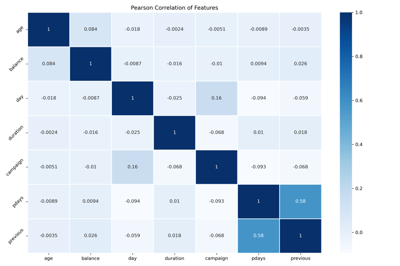
In this example, days and previous have the strongest correlation of 0.58, and everything else is independent of each other. A correlation of 0.58 isn't very strong. Therefore I will choose to leave both in the model.
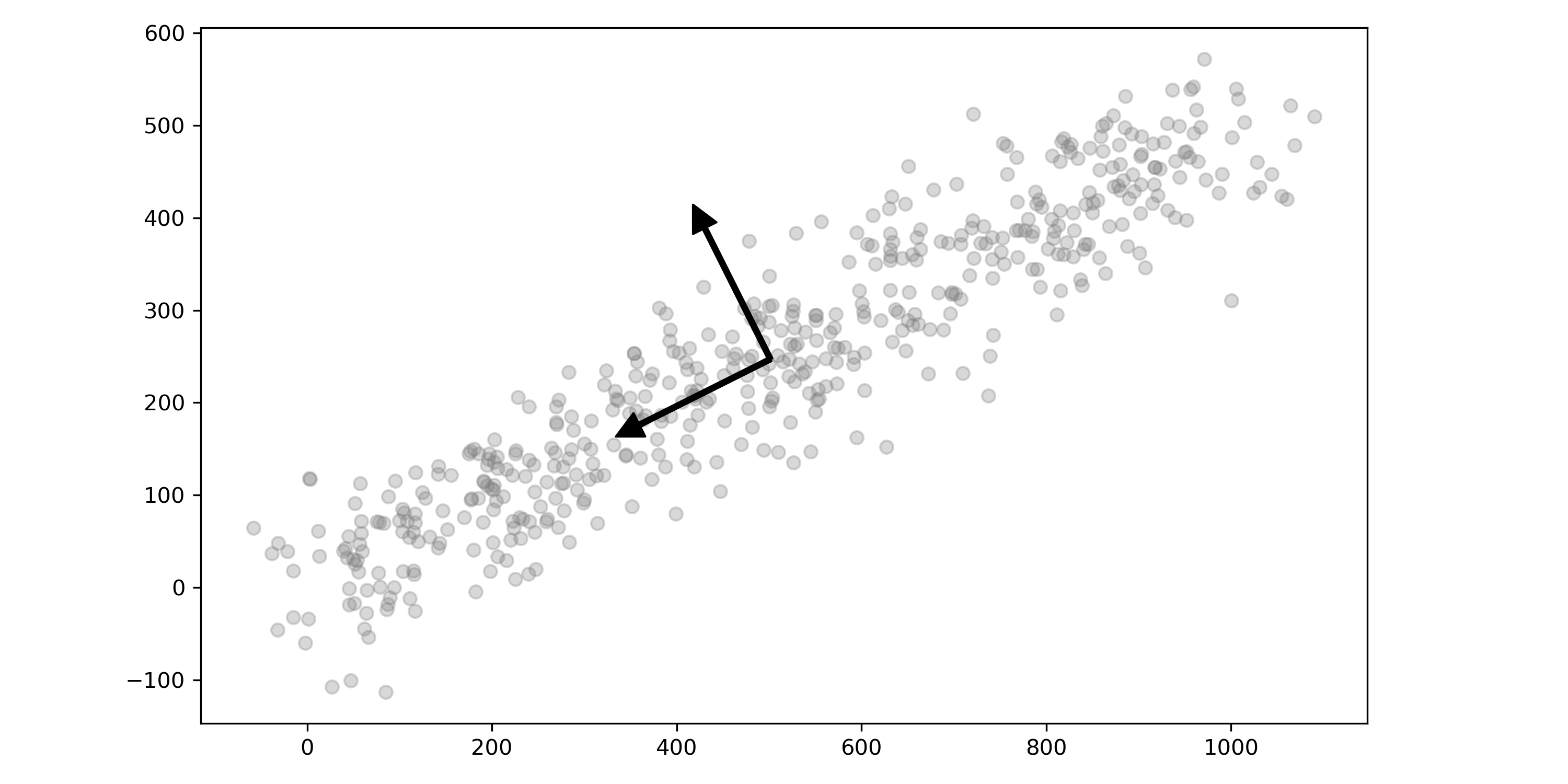
Principal Component Analysis
The most powerful method for feature selection in models where all of the data is numeric is Principal Component Analysis. PCA is not a feature selection method but a dimensionality reduction method. However, the objective with PCA is similar to Feature Selection, where we're looking to reduce the amount of data needed to compute the model.
The following image represents PCA applied to a photo. The plot represents the amount of cumulative explained variance for each principal component.

For more information on how PCA works and how to perform it, please review the following articles: 2 Beautiful Ways to Visualize PCA and The Magic of Principal Component Analysis through Image Compression
Feature Importance from Random Forests
Finally, my preferred method for feature selection is to utilize Random Forests and its ability to calculate Feature Importance. As an output of a trained model, Scikit-Learnand Random Forest can output the list of features and their relative contribution to the overall performance of a model. This method also works with other Bagged trees like Extra Trees and Gradient Boosting for classification and regression.
The bonus of this method is that it fits well with the overall flow of building a model. Let's walk through how this works. Let's start by getting all the columns from our Data Frame. Note that we can utilize both categorical and numeric data in this case.
print(df.columns)Index(['age', 'job', 'marital', 'education', 'default', 'balance', 'housing', 'loan', 'contact', 'day', 'month', 'duration', 'campaign', 'pdays', 'previous', 'poutcome', 'y'], dtype='object')
When reading the documentation for this dataset, you'll notice that the Duration column is something that we shouldn't use to train your model. We'll manually remove it from our list of columns.
Duration: last contact duration, in seconds (numeric). Important note: this attribute highly affects the output target (e.g., if duration=0, then y='no'). Yet, the duration is not known before a call is performed. Also, after the end of the call y is obviously known. Thus, this input should only be included for benchmark purposes and should be discarded if the intention is to have a realistic predictive model.
Additionally, we can remove any other features that might not be useful if we'd like. For our example, we'll keep all of them aside from duration.
# Remove columns from the list that are not relevant. targets = ['age', 'job', 'marital', 'education', 'default', 'balance', 'housing', 'loan', 'contact', 'day', 'month', 'campaign', 'pdays', 'previous', 'poutcome']
Next, we will utilize a Column Transfomer to transform our data into a machine learning acceptable format. I prefer to use pipelines whenever I build a model for repeatability. For more information on them, check out my article: Stop Building Your Models One Step at a Time. Automate the Process with Pipelines!.
For our transformation, I've chosen the MinMaxScaler for numeric features and the OrdinalEncoder encoder for categorical features. In the final model, I would most likely OneHotEncode (OHE) for the categorical features, but to determine feature importance, we don't want to expand the columns with OHE; we'll get more value out of treating them as one column with ordinal encoded values.
column_trans = ColumnTransformer(transformers=
        [('num', MinMaxScaler(), selector(dtype_exclude="object")),
        ('cat', OrdinalEncoder(), selector(dtype_include="object"))],
        remainder='drop')
Next, we create an instance of our classifier with a few preferred settings such as class_weight='balanced', which helps deal with imbalanced data. We'll also set the random_state=42 to ensure that we get the same results.
For more on imbalanced data, check out my article: Don’t Get Caught in the Trap of Imbalanced Data When Building Your ML Model.
# Create a random forest classifier for feature importance
clf = RandomForestClassifier(random_state=42, n_jobs=6, class_weight='balanced')

pipeline = Pipeline([('prep',column_trans),
                     ('clf', clf)])
Next, we'll split our data into training and test sets and fit our model to the training data.
# Split the data into 30% test and 70% training
X_train, X_test, y_train, y_test = train_test_split(df[targets],
                                   df['y'], test_size=0.3, random_state=0)

pipeline.fit(X_train, y_train)
We can call the feature_importances_ method against the classifier to see the output. Note how you reference the classifier in the pipeline by calling its name clf, similar to a dictionary in Python.
pipeline['clf'].feature_importances_
array([0.12097191, 0.1551929 , 0.10382712, 0.04618367, 0.04876248,
       0.02484967, 0.11530121, 0.15703306, 0.10358275, 0.04916597,
       0.05092775, 0.02420151])
Next, let's display these sorted by the greatest importance and their cumulative importance. The cumulative importance column is useful to visualize how the total adds up to 1. There is also a loop to cut off any feature that contributes less than 0.5 to the overall importance. This cutoff value is arbitrary. You could look for total cumulative importance of, say, 0.8 or 0.9. Play around with how your model performs with fewer or more features.
feat_list = []

total_importance = 0
# Print the name and gini importance of each feature
for feature in zip(targets, pipeline['clf'].feature_importances_):
    feat_list.append(feature)
    total_importance += feature[1]

included_feats = []
# Print the name and gini importance of each feature
for feature in zip(targets, pipeline['clf'].feature_importances_):
    if feature[1] > .05:
        included_feats.append(feature[0])

print('\n',"Cumulative Importance =", total_importance)

# create DataFrame using data
df_imp = pd.DataFrame(feat_list, columns =['FEATURE', 'IMPORTANCE']).\
                      sort_values(by='IMPORTANCE', ascending=False)
df_imp['CUMSUM'] = df_imp['IMPORTANCE'].cumsum()
df_imp
      FEATURE  IMPORTANCE    CUMSUM
1         job    0.166889  0.166889
0         age    0.151696  0.318585
2     marital    0.134290  0.452875
13   previous    0.092159  0.545034
6     housing    0.078803  0.623837
3   education    0.072885  0.696722
4     default    0.056480  0.753202
12      pdays    0.048966  0.802168
8     contact    0.043289  0.845457
7        loan    0.037978  0.883436
14   poutcome    0.034298  0.917733
10      month    0.028382  0.946116
5     balance    0.028184  0.974300
11   campaign    0.021657  0.995957
9         day    0.004043  1.000000
Finally, based on that loop, let's print out the features that we've selected overall. Based on this analysis, we removed about 50% of them from our model, and we can see which ones have the highest impact!
print('Most Important Features:')
print(included_feats)
print('Number of Included Features =', len(included_feats))
Most Important Features:
['age', 'job', 'marital', 'education', 'default', 'housing', 'previous']
Number of Included Features = 7
Thank you for reading! You can find all the code for this article on GitHub
Conclusion
Feature Selection is a critical part of the model building process, and it not only helps improve performance but also simplifies your model and its interpretation. We started out looking at how to utilize the Chi-Squared test for independence to select categorical features. Next, we looked at a Pearson's Correlation Matrix to visually identify highly correlated numeric features and also touched on Principal Component Analysis (PCA) as a tool to reduce dimensionality automatically on numeric datasets. Last, we looked at feature_importances_ from Random Forest as a way to select across both categorical and numeric values. We hope this gets you started on your journey to Feature Selection!