By
By
What is Hyperparameter Tuning?
Hyperparameter tuning is a method in which you finely tune a machine learning model. Hyperparameters are not specifically learned during the training process but can be adjusted to optimize how a model performs. Here are a few tips I like to think about when it comes to hyperparameter tuning:
- Hyperparameter tuning is generally the final step you should perform when building a model, right before the final evaluation.
- You will not get dramatically different results from tuning parameters. The biggest influences on a model's performance are feature selection and model selection.
- Hyperparameter tuning can assist with the generalization of a model, reducing overfit.
That being said, Tuning your model is an important step in the workflow. Here is a quick visual that might help you understand the process.
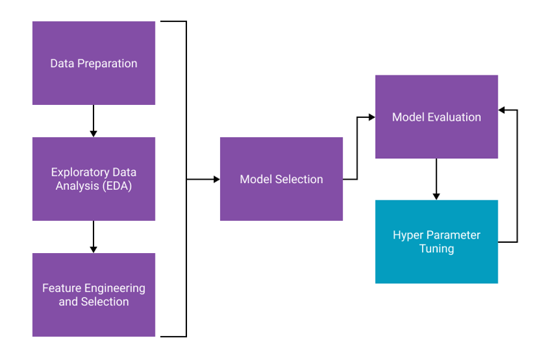
- Data Preparation: The process of cleaning your data and preparing it for machine learning.
- Exploratory Data Analysis: This is a step you should always perform. The process of exploring a new dataset and understanding data distributions, correlations, and more. See this post for a step-by-step guide.
- Feature Engineering and Selection: The process of creating new features (columns) from your data and choosing the best features based on how much they contribute to the model's performance.
- Model Selection: Utilizing cross-validation to choose which algorithm performs best based on an evaluation metric.
- Hyper Parameter Tuning: The process described in this post.
- Model Evaluation: Choosing the right performance metric and evlaulating results.
Examples of Hyper Parameters
Some examples of hyperparameters are:
- Which solver should I use in a logistic regression model?
- What is the best value for C, or the regularization constant?
- What regularization penalty should I use?
- What should be the maximum depth allowed for my decision tree?
- The number of trees should I include in my random forest?
Much of this could be very complex to figure out on your own. The good news is that you can apply various techniques to search for the optimal set of parameters. Now that you have a basic understanding of what they are and how they fit into the process let's look at how it works.
Model Selection
For brevity, we will skip the initial cleaning and feature selection. This code is available in this Notebook on GitHub. We'll take the results of our Feature Selection and create our Xand y variables.
X = df[['categories', 'postal_code', 'text_len', 'review_count', 'text_clean']]
y = df['target']
Next, we have a function that allows us to repeatably create a pipeline along with an instance of a classifier.
def create_pipe(clf, ngrams=(1,1)):

    column_trans = ColumnTransformer(
        [('Text', TfidfVectorizer(stop_words='english',
                                  ngram_range=ngrams), 'text_clean'),
         ('Categories', TfidfVectorizer(), 'categories'),
         ('OHE', OneHotEncoder(dtype='int',
                               handle_unknown='ignore'),['postal_code']),
         ('Numbers', MinMaxScaler(), ['review_count', 'text_len'])],
        remainder='drop')

    pipeline = Pipeline([('prep',column_trans),
                         ('over', SMOTE(random_state=42)),
                         ('under', RandomUnderSampler(random_state=42)),
                         ('clf', clf)])

    return pipeline
The pipeline contains all of the preprocessing steps required. Next, we can perform a classic Cross-Validation to find the best model.
models = {'RandForest' : RandomForestClassifier(random_state=42),
          'LogReg' : LogisticRegression(random_state=42)
          }

for name, model, in models.items():
    clf = model
    pipeline = create_pipe(clf)
    scores = cross_val_score(pipeline,
                             X,
                             y,
                             scoring='f1_macro',
                             cv=3,
                             n_jobs=1,
                             error_score='raise')

     print(name, ': Mean f1 Macro: %.3f and
           Standard Deviation: (%.3f)' % (np.mean(scores),
           np.std(scores)))
RandForest : Mean f1 Macro: 0.785 and Standard Deviation: (0.003)
LogReg : Mean f1 Macro: 0.854 and Standard Deviation: (0.001)
Overall, we can see that the LogisticRegression classifier performed better on this data than the RandomForestClassifier. As mentioned above, feature engineering, feature selection, and model selection will give you the biggest gains when training your model, so we always start here.
Accessing Model Parameters in a Pipelines
One of the first things I want to point out is how to access the parameters of a model in a pipeline. Normally, when you have an estimator (model) instance, you call estimator.get_params(), and you can see them. The process is the same in pipelines; however, the resulting output is slightly different.
When accessing parameters directly from an estimator, the output will be a value such as C. In contrast, in a pipeline, the output will first have the name you gave the estimator along with double-underscores and then finally the parameter name like clf__C; knowing how to access parameters is important since you need these names to build a parameter grid to search.
The following is the output from my pipeline, truncated for brevity. You can see at the end of the list the classifier parameters, all of which are currently the defaults.
pipeline.get_params()
{'memory': None,
 'steps': [('prep',
   ColumnTransformer(transformers=[('Text',
                                   TfidfVectorizer(stop_words='english'),
                                    'text_clean'),
                                   ('Categories', TfidfVectorizer(), 'categories'),
                                   ('OHE',
                                    OneHotEncoder(dtype='int',
                                                  handle_unknown='ignore'),
                                    ['postal_code']),
                                   ('Numbers', MinMaxScaler(),
                                    ['review_count', 'text_len'])])),

... truncated for brevity ...

 'clf__C': 1.0,
 'clf__class_weight': None,
 'clf__dual': False,
 'clf__fit_intercept': True,
 'clf__intercept_scaling': 1,
 'clf__l1_ratio': None,
 'clf__max_iter': 500,
 'clf__multi_class': 'auto',
 'clf__n_jobs': None,
 'clf__penalty': 'l2',
 'clf__random_state': 42,
 'clf__solver': 'lbfgs',
 'clf__tol': 0.0001,
 'clf__verbose': 0,
 'clf__warm_start': False}
Grid Search
The first method we'll explore is the Grid Seach Cross Validation which employs the same logic that we would use for regular cross-validation used for model selection. However, the Grid Search iterates through every combination of parameters and performs cross-validation, and returns the best model. The first step here is to create a parameter grid, and we do this by constructing a list of dictionaries for the GridSearch to iterate through.
parameters = [{'clf__solver' : ['newton-cg', 'lbfgs', 'sag', 'liblinear'],
               'clf__C' : [.1, 1, 10, 100, 1000],
               'prep__Text__ngram_range': [(1, 1), (2, 2), (1, 2)]}]
Alternatively, you can add more than one dictionary to the list. It will iterate through the combinations of each dictionary independently; useful if you have some parameters that are not compatible with others. For example, in LogisticRegression, certain penalty values only work with certain solvers.
parameters = [
  {'clf__penalty': ['l1', 'l2'], 'clf__solver' : ['liblinear']},
  {'clf__penalty': ['l1', 'none'], 'clf__solver' : ['newton-cg']},
  ]
Now that we have our parameter grid, we can first create an instance of our base classifier as well and pass that to our pipeline function.
clf = LogisticRegression(random_state=42, max_iter=500)
pipeline = create_pipe(clf)
Next we'll run the Grid Search with GridSearchCV.
%time grid = GridSearchCV(pipeline,
                          parameters,
                          scoring='f1_macro',
                          cv=3,
                          random_state=0).fit(X_train, y_train)

print("Best cross-validation accuracy: {:.3f}".format(grid.best_score_))
print("Test set score: {:.3f}".format(grid.score(X_test, y_test)))
print("Best parameters: {}".format(grid.best_params_))

log_C = grid.best_params_['clf__C']
log_solver = grid.best_params_['clf__solver']
log_ngram = grid.best_params_['prep__Text__ngram_range']
58m 3s

Best cross-validation accuracy: 0.867
Test set score: 0.872
Best parameters: {'clf__C': 100, 'clf__solver': 'newton-cg',
'prep__Text__ngram_range': (1, 2)}
Our grid search took 58m 3s to run, producing the best parameters for each.
One of the things that might jump out to you when looking at the above list is that there are quite a few potential combinations in our parameter grid. In the above example, there are 4x solver, 5x C, 3x n-grams, bringing the total to 4 x 5 x 3 = 60. Since training our model took about one minute, going through the grid once is linear to take about an hour.
Note: It's possible to parallelize the grid-search with the argument n_jobs=-1; however, I did not show the relative performance for this example.
Next, let's look at a way to improve the overall performance.
Halving Search
However, there is a way to speed up a GridSearch and return very similar results in much less time. The method is known as Successive Halving. It will utilize a subset of the data early in the process to find some of the best performing parameter combinations and gradually increase the amount of data used as it narrows in on the best combinations.
You can swap the GridSearchCV call with the HalvingGridSearchCV` call to utilize Halving Grid Search. Simple as that. Let's rerun the above search with this new approach and see how it performs.
%time grid = HalvingGridSearchCV(pipeline,
                                 parameters,
                                 scoring='f1_macro',
                                 cv=3,
                                 random_state=0).fit(X_train, y_train)


print("Best cross-validation accuracy: {:.3f}".format(grid.best_score_))
print("Test set score: {:.3f}".format(grid.score(X_test, y_test)))
print("Best parameters: {}".format(grid.best_params_))

log_C_b = grid.best_params_['clf__C']
log_solver_b = grid.best_params_['clf__solver']
log_ngram_b = grid.best_params_['prep__Text__ngram_range']
14m 28s

Best cross-validation accuracy: 0.867
Test set score: 0.872
Best parameters: {'clf__C': 100, 'clf__solver': 'lbfgs',
'prep__Text__ngram_range': (1, 2)}
Quite impressive! from an hour down to 15 minutes! In some cases, I've seen it perform even faster. We can also see that the results are quite similar. The solution selected was lbfgs this time versus newton-cg. We can compare the performance of both now.
Evaluating the Results
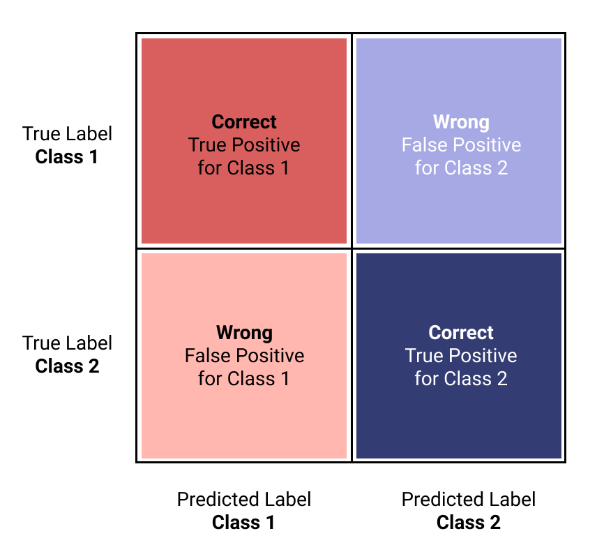
We have a simple function here that will take a pipeline, fit the data to a train and test set, and evaluate the results with a Classification Report and a Confusion Matrix. Let's successively go through the un-tuned model, the Grid Search tuned model, and finally, the Halving Grid Search tuned model. First up is the original model.
Note: The evaluation metric we're using here is F1-Macro; we are looking to balance out Precision and Recall.
def fit_and_print(pipeline, name):

    pipeline.fit(X_train, y_train)
    y_pred = pipeline.predict(X_test)
    score = metrics.f1_score(y_test, y_pred, average='macro')

    print(metrics.classification_report(y_test, y_pred, digits=3))

    ConfusionMatrixDisplay.from_predictions(y_test,
                                            y_pred,
                                            cmap=plt.cm.Greys)

    plt.tight_layout()
    plt.title(name)
    plt.ylabel('True Label')
    plt.xlabel('Predicted Label')
    plt.tight_layout()
    plt.savefig(name + '.png', dpi=300)
    plt.show;
clf = LogisticRegression(random_state=42, max_iter=500)
pipeline = create_pipe(clf)
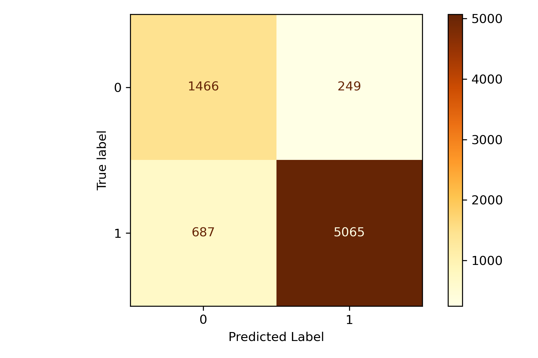
fit_and_print(pipeline, 'Default Parameters')
              precision    recall  f1-score   support

           0      0.789     0.845     0.816      9545
           1      0.925     0.894     0.909     20370

    accuracy                          0.879     29915
   macro avg      0.857     0.869     0.863     29915
weighted avg      0.882     0.879     0.880     29915

Our F1-Macro score here is 0.863. Next, let's try out the Grid Search tuned model.
clf = LogisticRegression(C=log_C, solver=log_solver, random_state=42, max_iter=500)
pipeline = create_pipe(clf, log_ngram)
fit_and_print(pipeline, 'GridSearch Parameters')
              precision    recall  f1-score   support

           0      0.839     0.810     0.824      9545
           1      0.913     0.927     0.920     20370

    accuracy                          0.890     29915
   macro avg      0.876     0.869     0.872     29915
weighted avg      0.889     0.890     0.889     29915
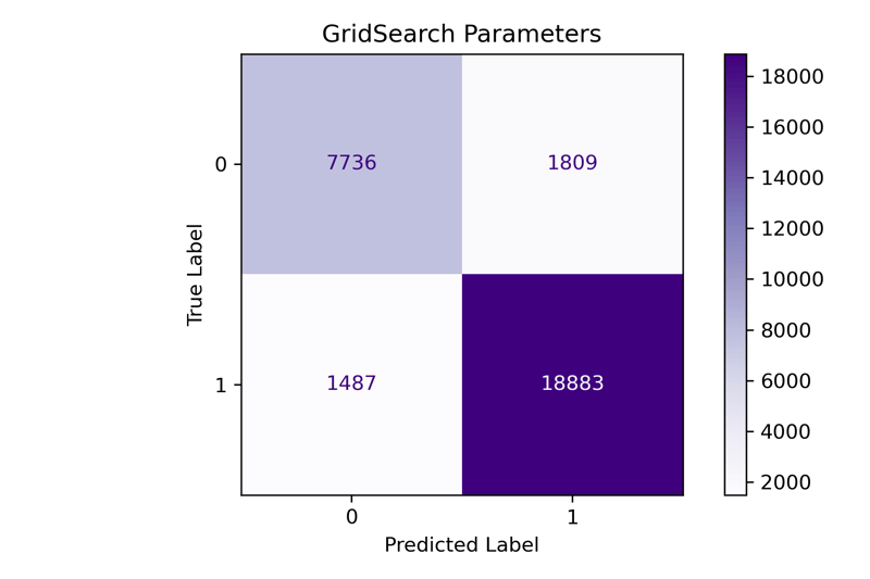
Our F1-Macro score here is 0.872. Our tuning process improved the overall results for the mode, and we increased the F1-Macro score by 0.09. Next, let's try out the Halving Grid Search tuned model.
clf = LogisticRegression(C=log_C_b,
                         solver=log_solver_b,
                         random_state=42,
                         max_iter=500)
pipeline = create_pipe(clf, log_ngram_b)
fit_and_print(pipeline, 'HalvingGridSearch Parameters')
              precision    recall  f1-score   support

           0      0.839     0.811     0.824      9545
           1      0.913     0.927     0.920     20370

    accuracy                          0.890     29915
   macro avg      0.876     0.869     0.872     29915
weighted avg      0.889     0.890     0.889     29915

Finally, we see the results of the Halving grid search model. The F1-Macro score is the same as the Grid Search model. We cut the time to tune from 60 minutes to 15 without sacrificing tuning results. Each time you utilize these methods, your results may vary, but it's an excellent way to tune a model without taking up a ton of your time.
Conclusion
Hyperparameter tuning is a way for you to tune your model after feature selection and model selection finely have been performed. Hyperparameters are not parameters learned during the training process but rather those adjusted to improve the overall performance of your model. We saw how to access parameters in a Pipeline and perform a Grid Search to select the best. Finally, you saw how you could utilize the Halving Grid search method to reduce the time it takes to search for the best parameters. I hope you enjoyed this article. Happy model building!
If you’d like to re-create this, all of this code is available in a Notebook on GitHub.