By
By
What is PCA?
Principal Component Analysis or PCA is a dimensionality reduction technique for data sets with many features or dimensions. It uses linear algebra to determine the most important features of a dataset. After these features have been identified, you can use only these features to train a machine learning model and improve performance without sacrificing accuracy. As a good friend and mentor of mine said:
"PCA is the workhorse in your machine learning toolbox."
PCA finds the axis with the maximum variance and projects the points onto this axis. PCA uses a concept from Linear Algebra known as Eigenvectors and Eigenvalues. There is a post on Stack Exchange which beautifully explains it.
Image Compression
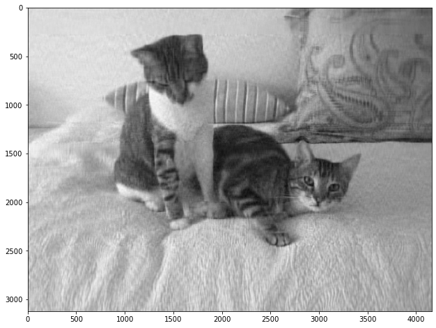
PCA is nicely demonstrated when it's used to compress images. Images are nothing more than a grid of pixels as well as a color value. Let's load an image into an array and see its shape. We'll use imread from matplotlib.
import numpy as np
import matplotlib.pyplot as plt
from matplotlib.image import imread

image_raw = imread("cat.jpg")
print(image_raw.shape)

plt.figure(figsize=[12,8])
plt.imshow(image_raw)
(3120, 4160, 3)
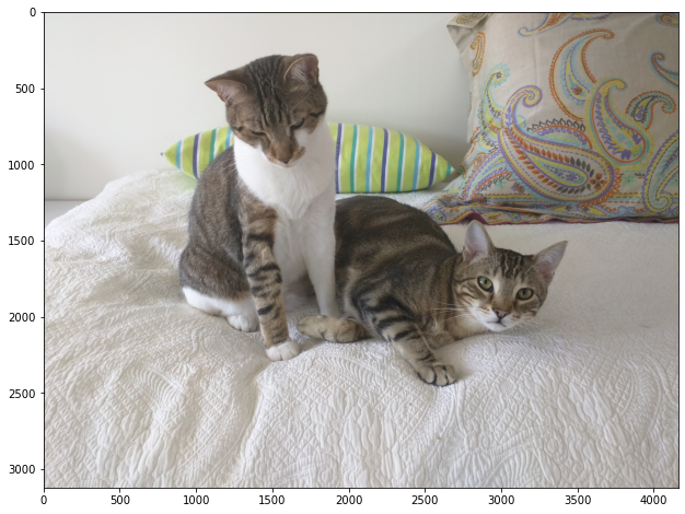
The results show a matrix of size (3120, 4160, 3). The first is the height of the image, the second is the width, and the third is the three channels of RGB values. Given the number of dimensions of this image, you can see how if you compared this to a classic tabular set of data, this would be considered quite large.
Before we continue, let's change this to a grayscale image to remove the RGB value.
# Show the new shape of the image
image_sum = image_raw.sum(axis=2)
print(image_sum.shape)

# Show the max value at any point.  1.0 = Black, 0.0 = White
image_bw = image_sum/image_sum.max()
print(image_bw.max())
(3120, 4160)
1.0
Calculating Explained Variance
Next we can fit our grayscale image with PCA from Scikit-Learn. After the image is fit, we have the method pca.explained_variance_ratio_ which returns the percentage of variance explained by each of the principal components. Utilizing np.cumsum we can add up each of the variance per component until it reaches 100% for the final component. We'll plot this on a line and show where 95% of explianed variace would be.
import numpy as np
from sklearn.decomposition import PCA, IncrementalPCA

pca = PCA()
pca.fit(image_bw)

# Getting the cumulative variance
var_cumu = np.cumsum(pca.explained_variance_ratio_)*100

# How many PCs explain 95% of the variance?
k = np.argmax(var_cumu>95)
print("Number of components explaining 95% variance: "+ str(k))
#print("\n")

plt.figure(figsize=[10,5])
plt.title('Cumulative Explained Variance explained by component')
plt.ylabel('Cumulative Explained variance (%)')
plt.xlabel('Principal components')
plt.axvline(x=k, color="k", linestyle="--")
plt.axhline(y=95, color="r", linestyle="--")
ax = plt.plot(var_cumu)
Number of components explaining 95% variance: 54
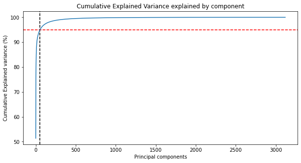
By printing off the length of components, we can see that there are 3120 components overall. I'm doing this to show how the number of components relates to the first value of our image matrix printed above.
len(pca.components_)
3120
What's crazy about this is that with PCA, we only need to use 54 of the original 3120components to explain 95% of the variance in the image! That's quite incredible.
Reducing Dimensionality with PCA
We'll use the fit_transform method from the IncrementalPCA module to first find the 54 PCs and transform and represent the data in those 54 new components/columns. Next, we'll reconstruct the original matrix from these 54 components using the inverse_transform method. And finally, we'll then plot the image to assess its quality visually.
ipca = IncrementalPCA(n_components=k)
image_recon = ipca.inverse_transform(ipca.fit_transform(image_bw))

# Plotting the reconstructed image
plt.figure(figsize=[12,8])
plt.imshow(image_recon,cmap = plt.cm.gray)
We clearly can see the quality of the image has been reduced, but it's still what the image is. From a Machine Learning perspective, training on this reduced set of data can produce nearly as good results but with fewer data.
Showing other Values for k-Dimensions
Next, let's iterative over six different k-values for our image, showing the progressively improving image quality at each number. We'll only go to 250 components, still just a fraction of the original image.
def plot_at_k(k):
    ipca = IncrementalPCA(n_components=k)
    image_recon = ipca.inverse_transform(ipca.fit_transform(image_bw))
    plt.imshow(image_recon,cmap = plt.cm.gray)

ks = [10, 25, 50, 100, 150, 250]

plt.figure(figsize=[15,9])

for i in range(6):
    plt.subplot(2,3,i+1)
    plot_at_k(ks[i])
    plt.title("Components: "+str(ks[i]))

plt.subplots_adjust(wspace=0.2, hspace=0.0)
plt.show()
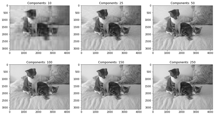
And that's it! As few as 10 components even lets us make out what the image is, and at 250 it's hard to tell the difference between the original image and the PCA reduced image.