By
By
What is Model Selection?
Model selection in Machine Learning is selecting the best model for your data. Different models will perform differently on different data sets and potentially by a large margin. It's pretty common these days that gradient boosted trees are the best performing models for tabular data, such as XGBoost, or the implementation in SciKit Learn. However, instead of always defaulting to a model such as XGBoost, it's important to evaluate the performance of different algorithms and see which one will perform the best for you.
Additionally, there can be some advantages to different models. For example, Logistic Regression can tell you the model's coefficients, allowing you to explain the impact of each feature on the final prediction. Bagged Tree Models like RandomForest can tell you the Feature Importance of each column in the model, similar to the coefficients of Logistic Regression.
Let's take a look at how to choose the best model across both a scoring metric of your choice as well as the speed of training.
Getting Started
For our demonstration today, we will use the Bank Marketing UCI dataset, which one can find on Kaggle. This dataset contains information about Bank customers in a marketing campaign, and it contains a target variable that one can utilize in a classification model. This dataset is in the public domain under CC0: Public Domain and can be used.
For more information on building classification models, check out: Everything You Need to Know to Build an Amazing Binary Classifier and Go Beyond Binary Classification with Multiclass and Multi-Label Models
We will start by importing the necessary libraries and loading the data. We'll be utilizing Scikit-Learn for our analysis today.
import numpy as np
import pandas as pd
import seaborn as sns
import matplotlib.pyplot as plt
from timeit import timeit

import warnings
warnings.filterwarnings('ignore')

from sklearn.model_selection import cross_val_score
from sklearn.model_selection import RepeatedStratifiedKFold
from sklearn.preprocessing import OneHotEncoder, LabelEncoder
from sklearn.preprocessing import MinMaxScaler
from sklearn.compose import ColumnTransformer

from sklearn.linear_model import LogisticRegression
from sklearn.linear_model import Perceptron
from sklearn.linear_model import SGDClassifier
from sklearn.tree import DecisionTreeClassifier
from sklearn.ensemble import RandomForestClassifier
from sklearn.ensemble import GradientBoostingClassifier
from sklearn.ensemble import HistGradientBoostingClassifier
from sklearn.ensemble import AdaBoostClassifier
from sklearn.ensemble import ExtraTreesClassifier
from sklearn.neighbors import KNeighborsClassifier
from sklearn.svm import SVC

from sklearn.compose import make_column_selector as selector
from sklearn.pipeline import Pipeline
Next, we'll load the data into a Pandas DataFrame and look at its shape.
df = pd.read_csv("bank.csv", delimiter=";")
df.shape
(4521, 17)
Data Cleaning
We have 4,500 rows of data with 17 columns including the target variable. We'll perform some light clean-up of the data before performing our model selection and first looking for null values, which there were none, and dropping any duplicates.
# check for nan/null
df.isnull().values.any()
# drop duplicates
len(df.drop_duplicates())
Next, in this particular dataset, we need to drop the column called duration. As stated in the documentation, this column has a large effect on the outcome of the target variable and, therefore should be excluded from training.
duration: last contact duration, in seconds (numeric). Important note: this attribute highly affects the output target (e.g., if duration=0 then y='no'). Yet, the duration is not known before a call is performed. Also, after the end of the call y is obviously known. Thus, this input should only be included for benchmark purposes and should be discarded if the intention is to have a realistic predictive model.
df.drop(columns='duration', inplace=True)
Data Preparation
Next, let's separate our data into X and y sets by utilizing simple python slicing. Since our target varable is the last column, we can simply take all but the last column for our Xdata and only the last column for our y data.
X = df.iloc[:, :-1]
y = df.iloc[:,-1]
Our y column is binary with yes and no values. It's best to encode these to 1 and 0utilizing the LabelEncoder from Skikit-Learn.
enc = LabelEncoder()
enc.fit(y)
y = enc.transform(y)
Next, we will utilize a Column Transfomer to transform our data into a machine learning acceptable format. I prefer to use pipelines whenever I build a model for repeatability. For more information on them, check out my article: Stop Building Your Models One Step at a Time. Automate the Process with Pipelines!.
For our transformation, we've chosen the MinMaxScaler for numeric features and an OneHotEncode (OHE) for the categorical features. OHE transforms categorical data into a binary representation, preventing models from predicting values between ordinal values. For more information on OHE, check out: One Hot Encoding.
column_trans = ColumnTransformer(transformers=
        [('num', MinMaxScaler(), selector(dtype_exclude="object")),
        ('cat', OneHotEncoder(), selector(dtype_include="object"))],
        remainder='drop')
Creating a List of Models for Model Selection
And now we're going to build a dictionary with our different models. Each entry in the dictionary consists of the name of the model as the Key and the pipeline as the Value.
The idea with model selection is to pick the best performing model, not tune the model for its best performance. That's known as Hyper Parameter Tuning, and you can read more about it here: 5-10x Faster Hyperparameter Tuning with HalvingGridSearch.
Because of this, we will simply instantiate each model with its default parameters. One exception is that I tend always to use the class_weight='balanced' parameter when available. It's a simple way to offset the issues you will have with imbalanced data. Read more about working with imbalanced data here: Don’t Get Caught in the Trap of Imbalanced Data When Building Your ML Model.
def get_models():
    models = dict()

    models['Logistic Regression'] = Pipeline([('prep', column_trans),
        ('model', LogisticRegression(random_state=42,
max_iter=1000, class_weight='balanced'))])

    models['Decision Tree'] = Pipeline([('prep', column_trans),
        ('model', DecisionTreeClassifier(random_state=42,
class_weight='balanced'))])

    models['Random Forest'] = Pipeline([('prep', column_trans),
        ('model', RandomForestClassifier(random_state=42,
class_weight='balanced'))])

    models['Extra Trees'] = Pipeline([('prep', column_trans),
        ('model', ExtraTreesClassifier(random_state=42,
class_weight='balanced'))])

    models['Gradient Boosting'] = Pipeline([('prep', column_trans),
        ('model', GradientBoostingClassifier(random_state=42))])

    models['Hist Gradient Boosting'] = Pipeline([('prep', column_trans),
        ('model', HistGradientBoostingClassifier(random_state=42))])

    models['AdaBoost'] = Pipeline([('prep', column_trans),
        ('model', AdaBoostClassifier(random_state=42))])

    models['SGD'] = Pipeline([('prep', column_trans),
        ('model', SGDClassifier(random_state=42,
class_weight='balanced'))])

    models['SVC'] = Pipeline([('prep', column_trans),
        ('model', SVC(class_weight='balanced', random_state=42))])

    models['Nearest Neighbor'] = Pipeline([('prep', column_trans),
        ('model', KNeighborsClassifier(3))])

    models['Perceptron'] = Pipeline([('prep', column_trans),
        ('model', Perceptron(random_state=42))])

    return models
Cross-Validation
It's critical when training a model that you do not overfit the model to your data or allow it to see all the data at once. Normally you would perform a train-test-split on your data; however, in this case, we're going to use a Cross-Validation approach to finding the best model utilizing the RepeatedStratifiedKFold method, which will handle partitioning the data into numerous train and test sets.
A Stratified sampling ensures that relative class frequencies are approximately preserved in each train and validation fold and is critical for imbalanced data. For more information on this method, check out: Cross-validation: evaluating estimator performance.
We'll build a reusable function that will allow us to test the different models we stored in our dictionary. There are a few parameters you can play with here, depending on your dataset size. You can determine the number of splits and repeats. If you have a smaller dataset like this example, try not to split your data too many times, or you won't have sufficient samples to train and test against.
Additionally, you need to specify the scoring metric you want to use. Scikit-Learn supports numerous different ones, and you can see how to reference them in their documentation. For this example, I've chosen ROC-AUC as my metric. For more information on choosing the best metric, check out: Stop Using Accuracy to Evaluate Your Classification Models.
# evaluate a give model using cross-validation
def evaluate_model(model, X, y):
    cv = RepeatedStratifiedKFold(n_splits=5,
                                 n_repeats=10,
                                 random_state=1)
    scores = cross_val_score(model, X, y,
                             scoring='roc_auc',
                             cv=cv, n_jobs=-1)
    return scores
Evaluating the Models
And now we can run our evaluation. We'll loop over our dictionary calling the evaluate_model function, and store the results in a list. We'll do the same for the model's name to make it simple for us to plot.
Each time the model is evaluated, we're also checking the speed of the model using the magic command %time, which prints out the time it took to evaluate the model, aiding our selection. We also print out the mean score and standard deviation of the scores for the ten repeats.
Finally, we'll plot the results on a single plot utilizing box-and-whiskers plots of the scores.
# get the models to evaluate
models = get_models()

# evaluate the models and store results
results, names = list(), list()
for name, model in models.items():
    %time scores = evaluate_model(model, X, y)
    results.append(scores)
    names.append(name)
    print('* %s Score = %.3f StdDev = (%.3f)' % (name,
np.mean(scores), np.std(scores)), '\n')

# plot model performance for comparison
plt.figure(figsize=(10,8))
plt.boxplot(results, labels=names, showmeans=True)
plt.xticks(rotation=45)
290 ms ± 0 ns per loop (mean ± std. dev. of 1 run, 1 loop each)
* Logistic Regression Score = 0.721 StdDev = (0.025)

204 ms ± 0 ns per loop (mean ± std. dev. of 1 run, 1 loop each)
* Decision Tree Score = 0.573 StdDev = (0.021)

1.61 s ± 0 ns per loop (mean ± std. dev. of 1 run, 1 loop each)
* Random Forest Score = 0.730 StdDev = (0.024)

1.68 s ± 0 ns per loop (mean ± std. dev. of 1 run, 1 loop each)
* Extra Trees Score = 0.701 StdDev = (0.021)

2.75 s ± 0 ns per loop (mean ± std. dev. of 1 run, 1 loop each)
* Gradient Boosting Score = 0.756 StdDev = (0.021)

2.04 s ± 0 ns per loop (mean ± std. dev. of 1 run, 1 loop each)
* Hist Gradient Boosting Score = 0.728 StdDev = (0.021)

886 ms ± 0 ns per loop (mean ± std. dev. of 1 run, 1 loop each)
* AdaBoost Score = 0.733 StdDev = (0.023)

212 ms ± 0 ns per loop (mean ± std. dev. of 1 run, 1 loop each)
* SGD Score = 0.690 StdDev = (0.031)

4.01 s ± 0 ns per loop (mean ± std. dev. of 1 run, 1 loop each)
* SVC Score = 0.715 StdDev = (0.027)

660 ms ± 0 ns per loop (mean ± std. dev. of 1 run, 1 loop each)
* Nearest Neighbor Score = 0.608 StdDev = (0.022)

127 ms ± 0 ns per loop (mean ± std. dev. of 1 run, 1 loop each)
* Perceptron Score = 0.639 StdDev = (0.043)
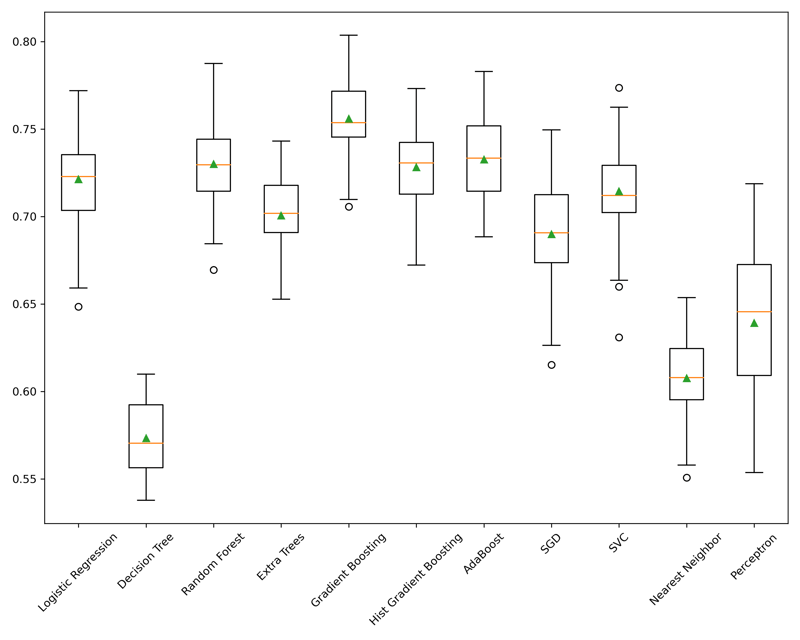
Here we get an excellent visual of each model's performance. Certain algorithms performed poorly, and we can discard them for this use case, such as the simple decision tree, the nearest neighbor classifier, and perceptron classifier. These are all some of the more simple models on the list, and it isn't a surprise that they performed poorer than the others. The Gradient Boosted Tree was the best performing classifier with a ROC-AUC score of 0.756, true to its reputation. AdaBoost and RandomForestwere the next best, with 0.733 and 0.730 scores, respectively.
We can also take a look at the time it took to run. Of these models, the Gradient Boosted Tree performed the slowest at 2.75 seconds, and AdaBoost the best of these at 886milliseconds. Look at Logistic Regression; however, it performed reasonably well at 0.721 but was extremely fast at 290 milliseconds which might weigh into our selection process. Logistic Regression has the advantage of high explainability by utilizing its coefficients and is performing at about 10% of the time of the Gradient Boosted Tree.
The final selection is up to you, but these methods should give you a strong baseline for how to select the best model for your use case!
All of the code for this article is available on GitHub
Conclusion
Model Selection is a critical step in your machine learning model building. Choosing the right model can greatly impact the performance of your machine learning model, and choosing the wrong model, can leave you with unacceptable results. We walked through the process of preparing our data by utilizing a Pipeline for consistency. We then built a list of models that we wanted to evaluate their performance. We utilized cross-validation to test each model on various data slices and finally plotted out the results. Utilizing this process is a quick and powerful way to select the right model for your application!