By
By
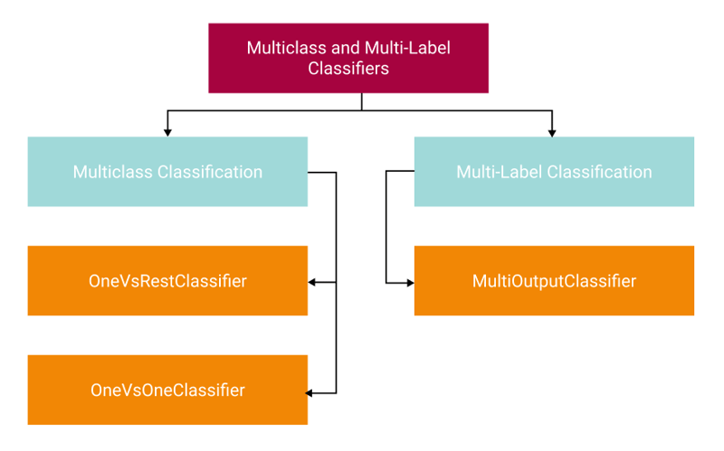
What are Multi-Class and Multi-Label Classification?
Often when you start learning about classification problems in Machine Learning, you start with binary classification or where there are only two possible outcomes, such as spam or not spam, fraud or not fraud, and so on. We have Multi-class and multi-labelclassification beyond that. Let's start by explaining each one.
Multi-Class Classification is where you have more than two categories in your target variable (y). For example, you could have small, medium, large, and xlarge, or you might have a rating system based on one to five stars. Each of these levels can be considered a class as well. The objective of this strategy is to predict a single class out of the available classes.
Multi-Label Classification is slightly different. Here you have more than two categories available as well, but instead of choosing only a single class, the objective of this strategy is to predict multiple classes when applicable. This strategy is useful when you have multiple categories related to each other. One of the best examples I've seen is when this is used in a tagging system. For example, Medium articles can have multiple tags associated with them. This particular article might have machine learning, data science, and python as tags.
Before you start, If you want a deep dive on Binary Classification, check out my article: Everything You Need to Know to Build an Amazing Binary Classifier
Now, let us dig into multi-class strategies.
Multi-Class Strategies
Strategies are how you approach instructing the classifier to handle more than two classes which may affect performance in terms of generalization or compute resources. Generalization refers to how well the classifier works on unseen data in the future; this is the opposite of overfitting. Check out the Scikit-Learn documentation for more information.
The One-vs-Rest or (OVR), also called One-vs-All (OVA) strategy, fits a single classifier for each class that is fitted against all other classes. OVR is essentially is splitting the multi-class problem into a set of binary classification problems. OVR tends to perform well because there are n classifiers for n classes. OVR is the most common strategy, and you can start here on your journey. What this looks like in practice is essentially this:
- Classifier 1: small vs (medium, large, xlarge)
- Classifier 2: medium vs (small, large, xlarge)
- Classifier 3: large vs (small, medium, xlarge)
- Classifier 4: xlarge vs (small, medium, large)
OVR tends to not scale well if you have a very large number of classes. One-vs-One might be better. Let's talk about that next.
The One-vs-One (OVO) strategy fits a single classifier for each pair of classes. Here is what that looks like:
- Classifier 1: small vs medium
- Classifier 2: small vs large
- Classifier 3: small vs. xlarge
- Classifier 4: medium vs large
- Classifier 5: medium vs xlarge
- Classifier 6: large vs xlarge
While the compute complexity is higher than the OVR strategy, it can be advantageous when you have a large number of classes because each of the classifiers is fit on a smaller subset of the data, where the OVR strategy is fit on the entire dataset for each classifier.
Finally for multi-label classification there is the MultiOutputClassifier. Similar to OVR, this fits a classifier for each class. However, as opposed to a single predicted output, this can, if applicable, output multiple classes for a single prediction.
Note: Specifically for the Scikit-Learn library, all classifiers are multi-class capable. You can use these strategies to refine their performance of them further.
Multi-Class Classification in Practice
Let's get started! Now that we understand some of the terminologies let's implement some strategies. For this example, we will use the dataset of Women’s E-Commerce Clothing Reviews on Kaggle, which is available for you to use under CC0: Public Domain. It's a set of review text, ratings, department names, and classes of each item. We're going to build a classifier that can predict the Department name based on the review text.
To begin, I like to use Pipelines to ensure repeatability of the process. A Pipeline allows you to transform your data into Machine learning suitable formats. We have two features that need transforming. We added the Review Text and a Text Length feature to the dataset. The Review Text will be vectorized utilizing TF-IDF and the second will use a MinMaxScaler to normalize the numerical data.
Note: There are a lot of steps missing in the process. Like importing data, text cleaning, and so on. Scroll to the end to get a link to this notebook on GitHub.
def create_pipe(clf):

    column_trans = ColumnTransformer(
            [('Text', TfidfVectorizer(), 'Text_Processed'),
             ('Text Length', MinMaxScaler(), ['text_len'])],
            remainder='drop')

    pipeline = Pipeline([('prep',column_trans),
                         ('clf', clf)])

    return pipeline
Next, we need to separate our data into the X data for learning and the target variable, y, which is how the model will learn the appropriate classes.
X = df[['Text_Processed', 'text_len']]
y = df['Department Name']
y.value_counts()
Tops        10048
Dresses      6145
Bottoms      3660
Intimate     1651
Jackets      1002
Trend         118
Name: Department Name, dtype: int64
We can see we're dealing with imbalanced data by checking the value_counts() for the target. The number of observations for the bottom few classes, especially Trend, is very small than the Tops class. We'll use a classifier that supports imbalanced data natively, but for a deep dive in working with imbalanced data, see my other post: Don’t Get Caught in the Trap of Imbalanced Data When Building Your ML Model.
Next, you should encode your target variable with the LabelEncoder. While Sklearn tends to handle text-based class names well, it's best to put everything into a numeric form before training.
le = LabelEncoder()
y = le.fit_transform(y)
le.classes_
array(['Bottoms', 'Dresses', 'Intimate', 'Jackets', 'Tops', 'Trend'],
      dtype=object)
By printing off the classes_, we can see which classes are encoded based on the order of the list.
Of course, when training our model, we need to split the dataset into Train and Test Partitions, allowing us to train our model and validate it on the test set to see how well it performs.
# Make training and test sets
X_train, X_test, y_train, y_test = train_test_split(X,
                                                    y,
                                                    test_size=0.33,
                                                    random_state=53)
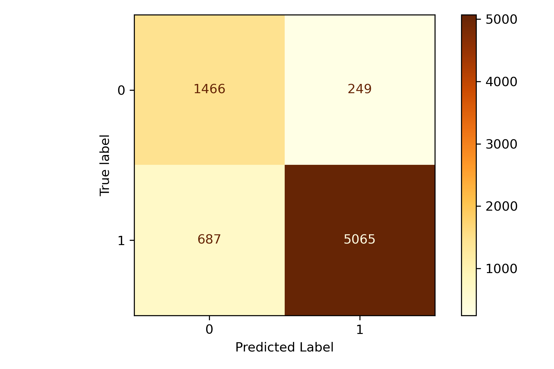
The next is a function to print off the classification report and a Confusion Matrix. Check out my article on how to best evaluate a classification model for more information: Stop Using Accuracy to Evaluate Your Classification Models
def fit_and_print(pipeline):

    pipeline.fit(X_train, y_train)
    y_pred = pipeline.predict(X_test)

    print(metrics.classification_report(y_test, y_pred, digits=3))

    ConfusionMatrixDisplay.from_predictions(y_test,
                                            y_pred,
                                            cmap=plt.cm.YlGn)

    plt.tight_layout()
    plt.ylabel('True label')
    plt.xlabel('Predicted Label')
    plt.tight_layout()
Here we're creating the instance of the classifier, fitting it, and evaluating it. We're using LogisticRegression, which is inherently a binary classifier. Sklearn has implemented multi-class directly as an argument of the classifier, but to demonstrate how One-vs-Rest works, I will use the wrapper instead. To accomplish this, you wrap your classifier with the OneVsRestClassifier() strategy I talked about above. This wrapper instructs the classifier on how to approach multi-class. We could also use the OneVsOneClassifierstrategy the same way. Go ahead and try both and compare the results.
clf = OneVsRestClassifier(LogisticRegression(random_state=42,
                                             class_weight='balanced'))
pipeline = create_pipe(clf)
fit_and_print(pipeline)
              precision    recall  f1-score   support

           0      0.785     0.855     0.818      1193
           1      0.905     0.844     0.874      2037
           2      0.439     0.581     0.500       527
           3      0.551     0.794     0.650       315
           4      0.909     0.818     0.861      3361
           5      0.022     0.061     0.033        33

    accuracy                          0.810      7466
   macro avg      0.602     0.659     0.623      7466
weighted avg      0.836     0.810     0.820      7466
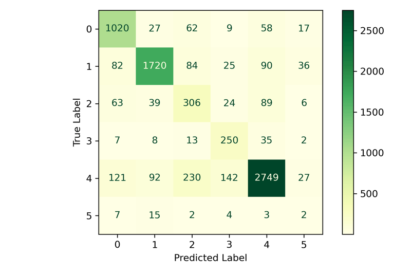
We can see that the model has the six classes listed with the relative performance of each class. The classes with larger counts performed quite well, while those with fewer were less. It will be impossible to generalize class 5 with so few observations. You might want to collect more data before training your model in real life.
Multi-Label Classification
Next, we'll look at a multi-label classification problem. We'll use the same dataset as before, but this time we'll use the Class Name as the target variable and a combination of the Review Text and Department Name as our features for learning. We start by creating our X and y data.
One special step we need to do this time is to tokenize the Class Name This is to ensure that when we binarize the text, we don't split the words into individual letters but rather maintain the full word as a whole.
# Tokenize the words
df['Class Name'] = df['Class Name'].apply(word_tokenize)
X = df[['Text_Processed', 'Department Name']]
y = df['Class Name']
To create a multi-label classifier, your target needs to be binarized into a multi-label format. In the above example, we used the LabelEncoder, which just converted the target class names to integers here; we'll use the MultiLabelBinarizer. If we print yafter the binarized is fit, we can see it results in a matrix of 0s and 1s. Anytime you pass a matrix (n-dimensional array) to a classifier (versus a vector, 1d array), it will automaticallybecome a multi-label problem.
mlb = MultiLabelBinarizer()
y = mlb.fit_transform(y)
print(y)
[[0 0 0 ... 0 0 0]
 [0 1 0 ... 0 0 0]
 [0 1 0 ... 0 0 0]
 ...
 [0 1 0 ... 0 0 0]
 [0 1 0 ... 0 0 0]
 [0 1 0 ... 0 0 0]]
mlb.classes_
array(['Blouses', 'Dresses', 'Fine', 'Intimates', 'Jackets', 'Jeans',
       'Knits', 'Layering', 'Legwear', 'Lounge', 'Outerwear', 'Pants',
       'Shorts', 'Skirts', 'Sleep', 'Sweaters', 'Swim', 'Trend', 'gauge'],
      dtype=object)
We can see the number of Classes is greater than the six Department Names we had above. Next, we'll create a Pipeline like before—however, we need to handle the department name differently this time. We're going to use the OneHotEncoder, which creates a new column in the DataFrame for each Class Name. The process marks each observation with a 0 or 1 depending on if the class name is in the row.
def create_pipe(clf):

    # Create the column transfomer
    column_trans = ColumnTransformer(
            [('Text', TfidfVectorizer(), 'Text_Processed'),
             ('Categories', OneHotEncoder(handle_unknown="ignore"),
              ['Department Name'])],
            remainder='drop')

    # Build the pipeline
    pipeline = Pipeline([('prep',column_trans),
                         ('clf', clf)])

    return pipeline
Similar to the above, we're going to wrap our classifier. This time we'll use the MultiOutputClassifier to instruct the classifier on how to handle the multiple labels. The rest of the process is the same.
clf = MultiOutputClassifier(LogisticRegression(max_iter=500,
                                               random_state=42))

pipeline = create_pipe(clf)

pipeline.fit(X_train, y_train)
y_pred = pipeline.predict(X_test)
score = metrics.f1_score(y_test,
                         y_pred,
                         average='macro',
                         zero_division=0)

print(metrics.classification_report(y_test,
                                    y_pred,
                                    digits=3,
                                    zero_division=0))
              precision    recall  f1-score   support

           0      0.691     0.420     0.523       973
           1      1.000     1.000     1.000      1996
           2      0.544     0.087     0.150       355
           3      1.000     0.019     0.036        54
           4      0.784     0.969     0.867       229
           5      0.943     0.676     0.788       340
           6      0.712     0.662     0.686      1562
           7      0.500     0.022     0.042        46
           8      1.000     0.174     0.296        46
           9      0.708     0.568     0.630       213
          10      0.875     0.393     0.542       107
          11      0.847     0.683     0.756       463
          12      0.765     0.263     0.391        99
          13      1.000     0.808     0.894       312
          14      1.000     0.039     0.076        76
          15      0.711     0.404     0.516       445
          16      0.958     0.590     0.730       117
          17      1.000     1.000     1.000        33
          18      0.544     0.087     0.150       355

   micro avg      0.844     0.640     0.728      7821
   macro avg      0.820     0.467     0.530      7821
weighted avg      0.812     0.640     0.688      7821
 samples avg      0.658     0.666     0.661      7821
Similar to the above, those with fewer observations per class will not perform as well, but those with a sufficient number tend to perform well. Let's take a look at what the classifier predicted.
We're going to add a column to our Test DataFrame by grabbing the predicted class names and then using the inverse_transform method from the MultiLabelBinarizerwe fit previously. We can add that as a column directly. To better demonstrate the results for this example, we will filter the DataFrame for only those observations with more than one label.
# Retreive the text labels from the MultiLabelBinarizer
pred_labels = mlb.inverse_transform(y_pred)
# Append them to the DataFrame
X_test['Predicted Labels'] = pred_labels

filter = X_test['Predicted Labels'].apply(lambda x: len(x) > 1)
df_mo = X_test[filter]
df_mo.sample(10, random_state=24)
                 Text_Processed Department Name         Predicted Labels
12561  cute summer blous top...            Tops         (Blouses, Knits)
15309  awesom poncho back ev...            Tops            (Fine, gauge)
6672   great sweater true fo...            Tops  (Fine, Sweaters, gauge)
4446   love top love fabric ...            Tops         (Blouses, Knits)
10397  love alway pilcro pan...         Bottoms           (Jeans, Pants)
14879  love shirt perfect fi...            Tops         (Blouses, Knits)
5948   simpl stylish top jea...            Tops         (Blouses, Knits)
16643  tri youll love beauti...            Tops  (Fine, Sweaters, gauge)
17866  qualiti sweater beaut...            Tops  (Fine, Sweaters, gauge)
22163  cute top got top mail...            Tops         (Blouses, Knits)
Awesome! You can see a bit of the text and the department name along with the Predicted Labels. If you look through the results, they seem to make sense as to what Classes might belong to Tops and Bottoms!
Conclusion
There you have it! Moving beyond binary classification takes a little extra knowledge to understand what is going on behind the scenes. Happy coding and classifying! There were a ton of steps I skipped, but I have all of them ready for you to use available on GitHub