By
By
What is Snowflake?
Snowflake is a cloud-based data platform designed to be easy to use and fast, and it is a fully managed which means there is no software to install or maintain. Snowflake has gained tremendous popularity due to its cloud-native approach, speed, and ease of use. Some of the world's largest companies use Snowflake, but any sized organization can also use it.
My favorite features of Snowflake are:
- Separation of storage and compute allows users to scale both resources dynamically and independently of each other.
- Flexible pricing model that allows users to pay for only the resources they use.
- Support for multiple public cloud providers like Amazon Web Services (AWS) or Microsoft Azure and Google Cloud Platform (GCP), which lets you run Snowflake in the same region as your other cloud services, saving you on networking costs.
- The ability to Time Travel allows you access to historical data where you can perform operations such as undrop a table that you accidentally deleted or even undo a query that updated data incorrectly.
- A unique Data Sharing feature allows you to share data with other users or organizations.
- A Marketplace full of data from third-party providers that you can use to enrich your warehouse.
In this post, I will show you how to get started with Snowflake and how to perform Extract, Load, and Transform (ELT) workflows.
What is ELT?
Traditionally, you loaded data into a data warehouse through a process called Extract, Transform, and Load or ETL. In the ETL process, you would extract data from a source system, transform it with external computing such as Apache Spark, and then load it into the warehouse in its final format.
With the rise of modern Data Warehouses like Snowflake, we invert the second and third parts of the process to perform Extract, Load, and Transform, known as ELT. In ELT, we extract data from a source system, load it into the warehouse, and then transform it. This process allows us to perform transformations in the warehouse, which can also be much faster than doing it in a separate computing engine. You also can reduce the complexity of your data pipeline by removing the need for an external computing engine.
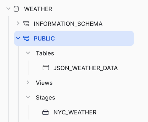
The load process happens in what is referred to as Stages. In Snowflake, the stage is in your database alongside the tables, views, etc.
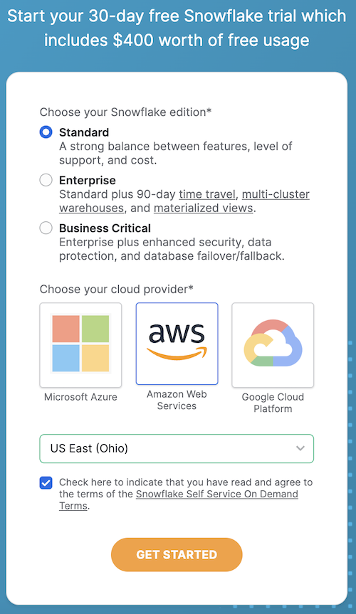
Create a Snowflake Trial Account
Head to the Snowflake and create a 30-Day Trial. After registering, you will need to choose a few basic things, such as the cloud provider of your choice and the region to run it in. No credit card information is needed unless you upgrade to a paid account.
Create a Warehouse
Next, we need to create a Warehouse. A warehouse in Snowflake terminology is not a place to store data, but rather the compute resources. Snowflake allows you to create multiple warehouses, allowing you to track different types of jobs and adjust the scale up and down for different types of jobs. For example, if you want to run a large ETL job, you can create a warehouse with many cores and then scale it down when the job is complete.
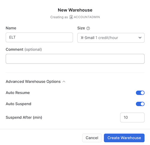
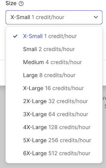
Note that in the drop-down for the size, it allows you to go from X-Small, which costs one credit per hour, up to the massive 6X-Large, which is a whopping 512 credits an hour! It's important to note that Snowflake supports auto-suspend and auto-resume. The warehouses will shut themselves down automatically when not used to avoid running up a bill when you're not doing work.
Putting it Into Practice
Go into the Worksheets section of the user interface and create a new worksheet where we will write our SQL queries. Snowflake saves your worksheets so you can come back to them at a later time. They're a great way to organize and track your work.
Run the following queries. Note that each has a semi-colon at the end of the line. If you don't put a semi-colon, Snowflake will execute the rest of the code below until it runs into the end of the file or another semi-colon.
We will create a database and set the warehouse to the one we created earlier. Next will tell Snowflake to use the database that was just created and then uses the publicschema, which was created by default.
Note: The data used in this example is provided as part of your Snowflake trial account.
create database weather;
use warehouse elt;
use database weather;
use schema public;
Once we have a database, we can create a table. We're going to create a single table with one column called v that is set to be a variant type, a special type in Snowflake that allows us to store any data. We're going to use this to store JSON data.
-- Note the variant type for JSON data.  V is the column name
create table json_weather_data (v variant);
Loading Data
Snowflake supports many different ways of loading data. One of the coolest and easiest ways is to pull in data directly from an S3 bucket. S3 is AWS's Simple Storage Service. It's a great way to store data in the cloud and is very common in industry workflows.
Now we can create our stage and set the source for the loading—a simple as these two lines of code to load your data into Snowflake.
-- Load the data from S3
create stage nyc_weather
url = 's3://snowflake-workshop-lab/zero-weather-nyc';
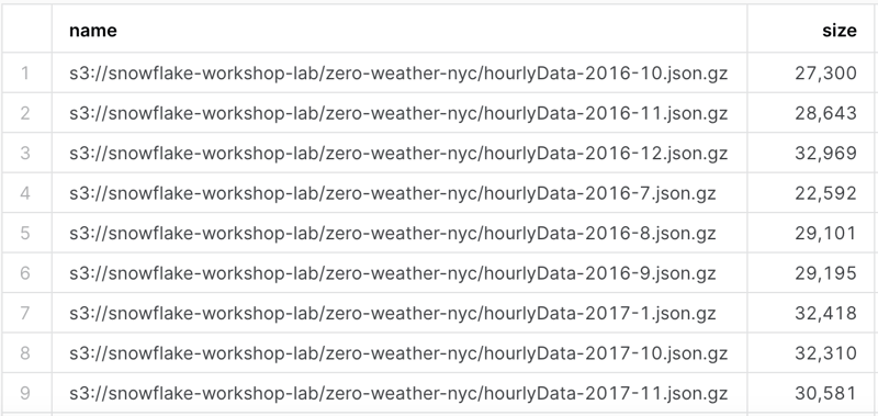
Next, we can use the list command with the @ symbol to list the files in the stage. Below we can see the list of files stored in the stage. Each is a JSON file with weather data in a compressed format (gz).
-- See what's in the stage
list @nyc_weather;
Now we need to move the data from the stage into the table. We can do this with the copy into command. We can also use the file_format option to specify the data format, which will do and tell the process to strip the outer array. Many JSON formats will start with [ and end with ]; in our use case, we won't need those. You can also create a custom file format that supports just about any file format you come across.
We'll also run a select statement to see the data in the table.
copy into json_weather_data
from @nyc_weather
    file_format = (type = json strip_outer_array = true);

select * from json_weather_data limit 10;
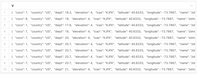
If we inspect a single entry from our v column, the JSON looks like the below snippet. While this is a great start, it doesn't help us with data analysis. We need to Transformthis data now into a tabular format.
{
  "coco": 7,
  "country": "US",
  "dwpt": 18.3,
  "elevation": 4,
  "icao": "KJFK",
  "latitude": 40.6333,
  "longitude": -73.7667,
  "name": "John F. Kennedy Airport",
  "obsTime": "2016-07-05T00:00:00.000Z",
  "prcp": 0,
  "pres": 1015.3,
  "region": "NY",
  "rhum": 76,
  "snow": null,
  "station": "74486",
  "temp": 22.8,
  "timezone": "America/New_York",
  "tsun": null,
  "wdir": 190,
  "weatherCondition": "Light Rain",
  "wmo": "74486",
  "wpgt": null,
  "wspd": 31.7
}
Transforming Data
This step next is how we're going to transform our data directly in Snowflake. This sample JSON data is fairly simple but will illustrate the point very well. Snowflake supports the ability to query JSON data directly in the database specifying key names in your query.
To make this data more accessible and always in a tabular format, we'll create a new View of this data based on the raw JSON data in our Table. That way, whenever the data is updated in the Table, the View will reflect the changes.
Note the syntax of the query. column:key_name::data_type. This pattern is repeated for each value we want to extract. We should also alias each of the columns with the askeyword to make them more readable.
-- create a view that will put structure onto the semi-structured data
create or replace view json_weather_data_view as
select
    v:obsTime::timestamp as observation_time,
    v:station::string as station_id,
    v:name::string as city_name,
    v:country::string as country,
    v:latitude::float as city_lat,
    v:longitude::float as city_lon,
    v:weatherCondition::string as weather_conditions,
    v:coco::int as weather_conditions_code,
    v:temp::float as temp,
    v:prcp::float as rain,
    v:tsun::float as tsun,
    v:wdir::float as wind_dir,
    v:wspd::float as wind_speed,
    v:dwpt::float as dew_point,
    v:rhum::float as relative_humidity,
    v:pres::float as pressure
from
    json_weather_data
where
    station_id = '72502';
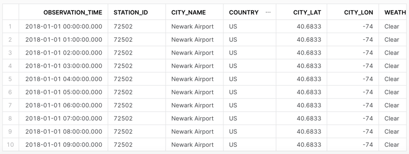
Now a select statement to query our new view will return a tabular data format.
select * from json_weather_data_view
where date_trunc('month',observation_time) = '2018-01-01'
limit 10;
That's it! We've now loaded, transformed, and queried our data in Snowflake. We can now use this data for analysis or visualization.
To see more on this workflow using data from MongoDB, check out my article How to Normalize MongoDB Data in Snowflake for Data Science Workflows and to run through the whole Snowflake quick start tutorial, visit Snowflake Quickstarts
Take it further and automate the workflow from an S3 bucket to a snowflake stage with Airflow. Check out my article Getting Started with Astronomer Airflow: The Data Engineering Workhorse for more details.
Conclusion
Snowflake is a cloud-native Data Warehouse solution built to scale from startups to enterprises. We talked about how modern data warehouses support the process of ELT or transform data directly in the Data Warehouse as an alternative to ETL. Next, we walked through loading data from an S3 Bucket into a Stage, then copying it into a Table. Finally, we showed Snowflake's powerful ability to query JSON directly and create columns from the keys. This article will hopefully give you a head start and on your way to new Data Engineering skills!