By
By
What Text Clustering?
In the last post, we talked about Topic Modeling, or a way to identify several topics from a corpus of documents. The method used there was Latent Dirichlet Allocation or LDA. In this article, we're going to perform a similar task but through the unsupervised machine learning method of clustering. While the method is different, the outcome is several groups (or topics) of words related to each other.
For this example, we will use the Wine Spectator reviews dataset from Kaggle1. It contains a little over 100,000 different wine reviews of varietals worldwide. The descriptions of the wines as tasting notes are the text-based variable that we're going to use to cluster and interpret the results.
Start by importing the needed libraries.
Note: I'm not going to show the preprocessing of the text here. You can see the full code on GitHub. There is also a full article on Text Cleaning you can reference.
from sklearn.feature_extraction.text import TfidfVectorizer
from sklearn.cluster import KMeans
from sklearn.metrics import silhouette_score

import matplotlib.pyplot as plt
import seaborn as sns
%matplotlib inline
Text Vectorizing
Vectorizing text is the process of converting text documents into numeric representations. There different versions of this, such as Bag-of-Words (BoW), as well as Term Frequency-Inverse Document Frequency (TF-IDF) which we'll be using here.
- BoW or TF: Represents the count of each word on a per-document basis. In this case, a document an observation in the data set of the column we're targeting.
- TF-IDF: Instead of just taking the count of words, it inverts this and gives a higher weighting to those words that appear less frequently. Common words have a lower weighting, whereas words that are probably more domain-specific and appear less will have a higher weighting.
It's quite easy to create the TF-IDF, create an instance of the vectorizer, and then fit-transform the column of the Data Frame.
 vectorizer = TfidfVectorizer()
X = vectorizer.fit_transform(df['description_clean'])
Determining the Best Number of Clusters
I mentioned above that clustering is an unsupervised machine learning method. Unsupervised means that we don't have information in our dataset that tells us the rightanswer; this is commonly referred to as labeled data. In our case, we don't know how many different types of wine there are or different topics discussed in the text. However, just because we don't know this information, it doesn't mean we can't find the right number of clusters.
With clustering, we need to initialize several cluster-centers. This number is fed into the model, and then after the results are outputted, someone with knowledge of the data can interpret those results. However, there are ways to evaluate which is the right number of cluster centers, and I'll cover two commonly used methods.
Elbow Method
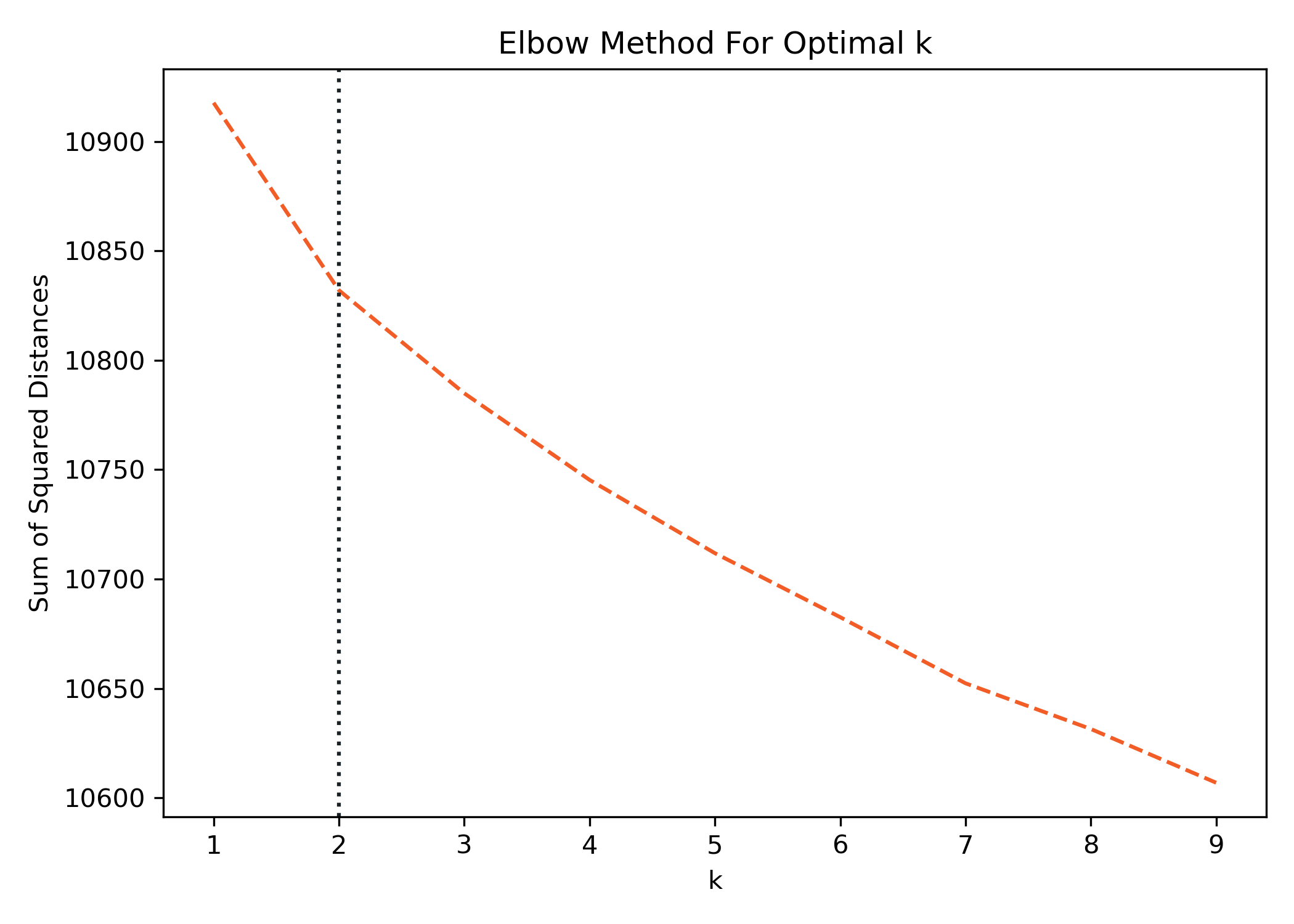
The first one is known as the Elbow Method. The name is derived from how the plot looks after running this analysis. Ideally, we're looking for a point where the curve starts to flatten out. This method uses inertia to determine the number of clusters. The inertia is the sum of the squared distances from each point to the cluster center. We can calculate this for a sequence of different cluster values, plot them, and look for the elbow.
 Sum_of_squared_distances = []
K = range(1,10)
for k in K:
    km = KMeans(init="k-means++", n_clusters=k)
    km = km.fit(X)
    Sum_of_squared_distances.append(km.inertia_)

ax = sns.lineplot(x=K, y=Sum_of_squared_distances)
ax.lines[0].set_linestyle("--")

# Add a vertical line to show the optimum number of clusters
plt.axvline(2, color='#F26457', linestyle=':')

plt.xlabel('k')
plt.ylabel('Sum of Squared Distances')
plt.title('Elbow Method For Optimal k')
plt.show()
The elbow isn't obvious after the data is plotted, but the best approximation is at 2 clusters where we see a slight kink in the curve. I've plotted a vertical line to identify it.
Silhouette Score
Another method for calculating the best cluster centers is the Silhouette Coefficient. The Silhouette Coefficient is calculated using the mean intra-cluster distance and the mean nearest-cluster distance for each sample. In other words, the distance between a sample and the nearest cluster that the sample is not a part of.
The best value is 1, and the worst is -1. Values near 0 indicate overlapping clusters. Negative values generally indicate that a sample has been assigned to the wrong cluster, as a different cluster is more similar versus the one it's assigned. Let's calculate these scores for various cluster centers values as well.
 def get_silhouette_score(X, k):
    for n_clusters in range(2, k):
        clusterer = KMeans(init="k-means++", n_clusters=n_clusters, random_state=42)
        y = clusterer.fit_predict(X)

        message = "For n_clusters = {} The average silhouette_score is: {}"
        print(message.format(n_clusters, silhouette_score(X, y)))

get_silhouette_score(X, 10)
 For n_clusters = 2 The average silhouette_score is: 0.00821919113279018
For n_clusters = 3 The average silhouette_score is: 0.006522933295313797
For n_clusters = 4 The average silhouette_score is: 0.006237960319271207
For n_clusters = 5 The average silhouette_score is: 0.006266850309331783
For n_clusters = 6 The average silhouette_score is: 0.006381665959703946
For n_clusters = 7 The average silhouette_score is: 0.005549433908077499
For n_clusters = 8 The average silhouette_score is: 0.005962146586290015
For n_clusters = 9 The average silhouette_score is: 0.00632540099660495
Per the definition, the number closest to 1 is the best, which in our case is 2 clusters. However, the values are close to zero, meaning our clusters have a high overlap.
While neither method gave us ideal visibility into the number of clusters, we should use, both point to 2 as the best value.
Clustering with k-Means
Okay! We're ready to build our model and check our results. This process is pretty straightforward, and we're going to repeat most of what we did above but on a single run with the number of clusters we've selected.
For this example, we're going to use k-Means. k-Means is one of the most common, if not the most common, clustering algorithms. Normally, k-Means will randomly initialize the cluster center and then iterate until it finds ideal locations. Specifying init="k-means++"means that we're going to use the k-means++ algorithm to initialize the cluster centers, which was proposed in 2007 as a way to reduce issues with random initialization3. I would suggest using this and reading up a little bit on how it works, for starters.
 # Set the number of clusters
k = 2
# Vectorize the text
vectorizer = TfidfVectorizer()
X = vectorizer.fit_transform(df['description_clean'])
# Fit our Model
model = KMeans(init="k-means++", n_clusters=k, max_iter=25, n_init=1)
model.fit(X)
You can save the cluster assignments as a new column in our data frame with the cluster numbers for future reference.
 # Get the cluster labels
clust_labels = model.predict(X)
cent = model.cluster_centers_

kmeans_labels = pd.DataFrame(clust_labels)
df.insert((df.shape[1]),'clusters',kmeans_labels)
And finally, let's build a quick data frame that shows the top 15 words from each of the two clusters and see what we get.
 order_centroids = model.cluster_centers_.argsort()[:, ::-1]
terms = vectorizer.get_feature_names_out()

results_dict = {}

for i in range(k):
    terms_list = []

    for ind in order_centroids[i, :15]:
        terms_list.append(terms[ind])

    results_dict[f'Cluster {i}'] = terms_list

df_clusters = pd.DataFrame.from_dict(results_dict)
df_clusters
     Cluster 0   Cluster 1
0   pineapple      cherry
1      flavor      flavor
2     acidity         dry
3     vanilla  blackberry
4       fruit      tannin
5         oak        cola
6       crisp   raspberry
7        pear     currant
8       apple        good
9       peach        rich
10       lime        soft
11     butter       spice
12      toast        show
13      sweet         oak
14      lemon       sweet
Looking at cluster 0, we see words typically associated with White wines, and cluster 1are associated with Red.
Predicting New Docs
Next, we can see how the model would cluster new wine reviews that it's not seen in the past. I've made up a few sentences that use words that white and red wines might have associated with them.
 new_docs = ['Rich deep color of oak and chocolate.',
            'Light and crisp with a hint of vanilla.',
            'Hints of citrus and melon.',
            'Dark raspberry and black cherry flavors.']

pred = model.predict(vectorizer.transform(new_docs))
print(pred)
[1 0 0 1]
The red wines are classified as 1 and whites as 0 exactly as we would expect! You can play around with other strings and see how it performs.
Conclusion
The first time I performed clustering on this dataset, I was honestly blown away. It was so obvious that with 2 clusters, the algorithm identified and clustered red versus white wines. It felt a little like magic, but in the end, it's just math! Enjoy playing with this process. It's powerful and can help you identify related groups of topics in your text!