By
By
What is a Marketing Attribution Platform?
A Marketing Attribution Platform is a tool that allows you to track the effectiveness of your marketing campaigns. It does this by tracking the user's journey from the first time they visit your site to the point of conversion.
Lassoo is a Marketing Attribution Platform with a couple of huge advantages. Not only does it make it easy to instrument your site with a point-and-click interface, but the data is also organized so that it's incredibly clean and easy to build Machine Learning models. In many cases, all the features you would need to create are already available, and it even has binary classification targets pre-built into the data. In this article, I'll show you how to leverage Lassoo to build a model that predicts which users will convert to paid.
Motivation
This article will focus less on the fundamentals of model building and more on the overall methodology in setting up the end-to-end process for moving this into production. There will be references to best practices throughout as needed.
I am going to break this down into three steps:
- Step 1: Creating Production-Ready Queries for Our Model
- Step 2: Model Building with XGBoost
- Step 3: Inferencing on Fresh Data
In each of these steps, I'll explain the thought process and logic behind the steps.
Let's go!
Step 1: Creating Production-Ready Queries for Our Model
One of the goals was to create queries that included all of the selected features needed plus all feature engineering already performed. By doing this, we can avoid a lot of cleanup when we inference new data. I'll show the inferencing at the end of this article, demonstrating how simple it is to build clean queries from the start.
The product has great documentation for direct SQL access, which I'll use below. By giving you direct SQL access, as a Data Scientist, you instantly are comfortable working with this data.
Keeping Your Dataset Balanced
I know from investigating this dataset that we have very imbalanced data. Imbalanced data is a common situation where fewer people have purchased products that have yet to. I also know that this is a very large dataset. I wanted to develop an approach for training that would allow me to take a subset of the data but preserve the class balance.
I'll start by getting the counts of each class for the window of time that I intend to train my data on (which is essentially six months of data. More on that shortly.) I'm also utilizing a date-based constraint where I'm fetching data where the user's last_seendate is older than seven days but later than six months. In cases like this model, trying to predict purchase behavior, we want to stay within our data since multiple things could have changed, such as ad campaigns, product offerings, and more. With Postgres, I can use the INTERVAL function to do this easily.
true_counts = """
SELECT COUNT(*)
FROM person_""" + tf_api + """ P
WHERE (P.has_purchased is True)
AND (P.last_seen < CURRENT_DATE - INTERVAL '7 days')
AND (P.last_seen > CURRENT_DATE - INTERVAL '6 months');
"""
I ended up with 46,5998 for the true_counts and 2,759,986 for the false_counts. I'll use 25% of these as limits stored in a variable for the queries below.
df_true = pd.read_sql(true_counts, dbConnection);
lim_true = int(df_true.iloc[0,0] * .25)
lim_true
Building ML-Ready Queries
We have three nearly identical queries. The first two segments out data for both classes, and the final data is people who have yet to purchase that we want to predict their behavior.
person_purchased- People who have purchased in the past six months. We will use this to train/test our model.person_not- People who have not purchased in the past six months. We will use this to train/test our model.person_test- People who have not purchased but visited the site within the last seven days. We'll use this as our final validation set that we'll infer.
Feature Engineering
Before we explore the queries, I want to cover how Feature Engineering is built right into the query itself, as opposed to doing this during model building.
Why is this critical, and how did I arrive here?
First of all, I performed all of the Exploratory Data Analysis and Feature Engineering inside my model building notebook. I also performed Feature Selection, running the model multiple times until I settled on the last data I wanted.
I won't show that below because after I performed all these steps, I built that directly into the SQL query statements. What this allows me to do, is completely skip this step later when it comes to model inference on new data! A huge time saver and improves the overall robustness of the model. Let's take a look at a few steps.
EXTRACT(EPOCH FROM (P.last_seen - P.first_seen)): This select statement calculates the number of seconds between thelast_seendate and thefirst_seendate. This calculation is useful in determining how long a user has been visiting the site. Also, utilizing EPOCH time instead of Date Diff is easier since everything is normalized to several seconds. When utilizing Date Diff, you can run into some in days; some are in milliseconds, making it something you must process again to normalize.count(distinct),sum(), andavg()are all aggregate functions performed on the session table`: This is a great way to get a sense of how many times a user has visited the site, how many times they've clicked on a link, how many times they've input data, etc. You could reserve aggregations for Pandas, but it's much more efficient (and easier) to do right in your query.P.multi_device::intandP.has_purchased::int; this operation casts a boolean value as an integer. Most ML models need to work with integer values, and getting these into the correct format is easier before moving forward.
You can extend this concept further with all of your feature engineering needs. I recommend doing it this way.
Extracting the Data for Specific Date Windows
Now let's run the actual queries that will extract our data. As mentioned above, we don't want to go back too far in time with our data, so we'll implement the same date window constraint we used for the counts above.
Two additional notes. First, I'm utilizing the function RANDOM() on the ORDER BY clause so that we return a random subset of data instead of something ordered. Remember, we're only pulling 25% of the total data available. Second, I've inserted the variable str(lim_true) into the LIMIT clause, or the variable we created earlier that holds the limit for the number of records we want to return.
Eventually, we will have to re-train our model due to drift. Drift is the concept of our model's performance decaying over time due to the natural changes in the dataset. The same is why we selected a trailing six-month window for training. If we re-train the model by re-running the queries, we'll get a new set of data that's in line with the current date!
person_purchased = """
SELECT
P.person_id,
P.first_utm_medium,
P.first_utm_source,
P.multi_device::int,
P.session_count,
P.last_utm_medium,
P.last_utm_source,
P.source_category,
P.source_category_2,
P.source_category_3,
EXTRACT(EPOCH FROM (P.last_seen - P.first_seen)) as since_first_vist,
count(distinct S.first_utm_content) as first_utm_content_distinct,
count(distinct S.first_utm_medium) as first_utm_medium_distinct,
count(distinct S.first_utm_source) as first_utm_source_distinct,
count(distinct S.first_utm_term) as first_utm_term_distinct,
sum(S.click_count) as click_count_sum,
sum(S.input_count) as input_count_sum,
sum(S.identify_count) as identify_count_sum,
sum(S.view_count) as view_count_sum,
sum(S.page_count) page_count_sum,
count(distinct S.source_category) as source_category_distinct,
avg(S.session_duration) as session_duration_avg,
P.has_purchased::int
FROM person_""" + tf_api + """ P
JOIN session_""" + tf_api + """ S
ON S.person_id = P.person_id
WHERE (P.has_purchased is True)
AND (P.last_seen < CURRENT_DATE - INTERVAL '7 days')
AND (P.last_seen > CURRENT_DATE - INTERVAL '6 months')
GROUP BY P.person_id
ORDER BY random()
LIMIT """ + str(lim_true) + ';'
Then repeat the above for the false_counts replacing WHERE (P.has_purchased is True) with False and LIMIT """ + str(lim_true) with str(lim_false).
Now that we have our data representing our two classes let's build a set of data that's unseen by the model. In this case, we'll take data where the user's last seen value is greater than seven days ago. We'll keep the number of records here as we did above. We'll take all users who haven't purchased but have visited in the last seven days.
person_test = """
SELECT ... (same as above)

WHERE (P.has_purchased is False)
AND (P.last_seen > CURRENT_DATE - INTERVAL '7 days')
GROUP BY P.person_id;
"""
Now we can check the shape of our data frames and persist them into .pkl files to make the data easier to work with without running the queries again.
print(df_purchased.shape)
print(df_not.shape)
print(df_test.shape)
(116483, 23)
(689983, 23)
(265888, 23)
We have 116k records for our purchased class, 690k for our not purchased class, and 266k for our validation set. Check out the entire process and code for this portion on GitHub.
Step 2: Model Building with XGBoost
Now that we have our data let's build a model. We'll be using the XGBoost library. XGBoost is a gradient-boosting library that is very popular in the ML community. It's a great library to start with and is very easy to use. It's also very fast and can be used for classification and regression problems. In most cases with tabular data, it's safe to assume that XGBoost will be a good choice. Note: I did perform Model Selection and XGBoost was the best performing model.
Another huge advantage of XGBoost is that it natively handles null values. We don't have to worry about imputing missing values, and we can leave them as null, and XGBoost will handle them for us.
Let's start by loading our data. Because we have two different classes, each with its file, we'll import their data frame. Then, we'll utilize the contact method to combine the two data frames.
df1 = pd.read_pickle('person_purchased.pkl')
df2 = pd.read_pickle('person_not.pkl')
df = pd.concat([df1, df2], axis=0)
df.shape
(806466, 23)
We'll also check the value_counts for our target variable; of course, they match the data set sizes we extracted earlier.
df["has_purchased"].value_counts()
0    689983
1    116483
Model Training
Next, we can train our model. We first split our dataset into X and y partitions. Let's start by inspecting a single data record to see how it looks after our query did all the work to build our features.
We can see a handful of categorical values such as first_utm_medium and first_utm_source and our aggregate values like click_count_sum and session_duration_avg—clean, nice features.
df_X.iloc[1]
first_utm_medium               google_ads
first_utm_source                   search
multi_device                            0
session_count                           5
last_utm_medium                google_ads
last_utm_source                   display
source_category               Paid Search
source_category_2                 Branded
source_category_3                    None
since_first_vist              20218985.28
first_utm_content_distinct              1
first_utm_medium_distinct               1
first_utm_source_distinct               2
first_utm_term_distinct                 1
click_count_sum                        48
input_count_sum                         4
identify_count_sum                      2
view_count_sum                          1
page_count_sum                         72
source_category_distinct                4
session_duration_avg                  4.6
Name: 0, dtype: object
I always utilize Pipelines when building my models. In this case, it's critical since we'll be persisting our model to disk, and we want to ensure the data transformations are included in the pipeline for when we perform our inferences on new data.
Our Pipeline contains two different transformers. First, a MixMaxScaler will scale all numeric data between 0 and 1. Second is our OneHotEncoder which will take categorical values and convert them into their columns for each value, a critical best practice for ML Model building.
def create_pipe(clf):

    column_trans = ColumnTransformer(transformers=
        [('num', MinMaxScaler(), selector(dtype_include='number')),
         ('cat', OneHotEncoder(dtype='int', handle_unknown='ignore'), \
            selector(dtype_include="object"))],
        remainder='passthrough', verbose_feature_names_out=True)

    pipeline = Pipeline([('prep',column_trans), ('clf', clf)])

    return pipeline
And now, create our instance of the XGBClassifier. We could perform Hyperparameter Tuning here; however, we'll use some of the more robust defaults for XGBoost for starters.
clf = xgb.XGBClassifier(random_state=42,
                        verbosity=0,
                        objective='binary:logistic',
                        scale_pos_weight=estimate,
                        n_estimators=1000,
                        max_depth=6,
                        learning_rate=0.5)

pipeline = create_pipe(clf)
And now, we can fit our model into our training data.
pipeline.fit(X_train, y_train)
We can utilize the feature_importances_ to see how much weight each feature has on our model; a great way to introduce Explainability into our process, where we can describe to business stakeholders how our model is making decisions.
feat_list = []
xgb_cols = get_feature_names(pipeline['prep'])
feat_imp = pipeline['clf'].feature_importances_

total_importance = 0
# Print the name and gini importance of each feature
for feature in zip(xgb_cols, feat_imp):
    feat_list.append(feature)
    total_importance += feature[1]

# create DataFrame using data
df_imp = pd.DataFrame(feat_list, columns =['FEATURE', 'IMPORTANCE']).\
sort_values(by='IMPORTANCE', ascending=False)
df_imp['SUMMED_TOTAL'] = df_imp['IMPORTANCE'].cumsum()
df_imp.head(10)
                              FEATURE  IMPORTANCE  SUMMED_TOTAL
9             num__identify_count_sum    0.551607      0.551607
82        cat__first_utm_source_email    0.031941      0.583548
214  cat__source_category_Paid Search    0.028456      0.612005
196         cat__last_utm_source_sfmc    0.025089      0.637093
49        cat__first_utm_medium_email    0.025076      0.662169
182        cat__last_utm_source_email    0.014413      0.676583
11                num__page_count_sum    0.012657      0.689239
211        cat__source_category_Email    0.009739      0.698978
210      cat__source_category_Display    0.008529      0.707508
8                num__input_count_sum    0.007481      0.714989
Here we see the top 10 features sorted by their contribution (IMPORTANCE) and cumulative total. Our first feature, num__identify_count_sum, is the most important in our model, contributing 55% of the overall importance. Next is cat__first_utm_source_email, contributing 3.2% to the model. The top 10 features contribute 71% of the overall importance. We can also learn information such as the email method of first contact is effective, and so is Paid Search.
Evaluating our Model
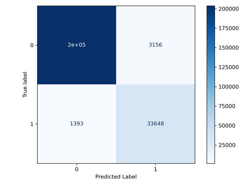
Finally, we want to see how our model is performing overall. We utilize a Confusion Matrix to help us identify how our classifier performs on each class.
def print_confusion(pipeline):
    ''' take a supplied pipeline and run it against the train-test spit
    and product scoring results.'''

    y_pred = pipeline.predict(X_test)

    print(metrics.classification_report(y_test, y_pred, digits=3))

    ConfusionMatrixDisplay.from_predictions(y_test,
                                            y_pred,
                                            cmap=plt.cm.Blues)

    plt.tight_layout()
    plt.ylabel('True label')
    plt.xlabel('Predicted Label')
    plt.tight_layout()
    plt.savefig('02_confusion_matrix.png', dpi=300);
We can see from the following output that our model performs very well on our test data. Since we have imbalanced data, we should never use the metric Accuracy but rather precision, recall, or f1 score. We'll use f1 to balance precision and recall for class 1. Our model is performing very well with an f1 score of 0.937*.
print_confusion(pipeline)
              precision    recall  f1-score   support

           0      0.993     0.985     0.989    206899
           1      0.914     0.960     0.937     35041

    accuracy                          0.981    241940
   macro avg      0.954     0.972     0.963    241940
weighted avg      0.982     0.981     0.981    241940
Persisting the Model
To run this in production, we need to persist our model on disk so that we can load it easily. We can accomplish this with the joblib library.
dump(pipeline, '02_tf_first_purchase.joblib')
Next up, let's run this on our "new" production data!
You can find all of the code for this portion of the process on GitHub
Step 3: Inferencing on Fresh Data
The final step in our process is loading our model from disk and inferencing new data against it. We'll use the joblib library to load our model from disk and then use the predict_proba method to get the purchase probability for each row in our dataset.
The beautiful part of this process is the performance. We can load the model and run it against 265k records in about 1 second. Incredible performance and efficiency allow us to do this daily.
We'll start by loading only pandas and joblib libraries.
import pandas as pd
from joblib import load
Then we can load our data from our .pkl file. Ideally, we might pull this data out of a database or object store (like AWS s3), but the pickle file will suffice for this example.
We also load the model using the load method from joblib. I name it pipeline because we're loading our trained model and the entire pipeline that fits our training data, including both the transformers and the classifier.
df = pd.read_pickle('person_test.pkl')
pipeline = load('02_tf_first_purchase.joblib')
Next, we can separate the target from the rest of the data for cleanliness. We'll then utilize the predict_proba method to get the purchase probability for each row in our dataset. We'll then add the probability to our data frame and sort it by the highest purchase probability.
The probability will be from 0 to 1. By default, anything above 0.5 is a purchase, and anything below 0.5 is not a purchase.
X = df.drop(columns=['has_purchased']).copy()
y = df['has_purchased'].copy()

# Predict the outcome variable based on the model
probs = pipeline.predict_proba(X)

# Get the Win probability for the `win` class
probs = probs[:,1]
probs = probs.round(3)

# Add the probability percentage to the DataFrame
X['last_prediction_date'] = pd.Timestamp.today().strftime('%Y-%m-%d')
X['convert_probability'] = probs.tolist()
Because 50% probability might leave us with some customers that are borderline likely to purchase, we can adjust the threshold to only include customers with some percentage of likeliness to purchase. In this case, we'll only include customers with a probability of 75% or higher.
df_probs = X.sort_values('convert_probability', ascending=False)
df_leads = df_probs[df_probs['convert_probability'] >= 0.75]
df_leads[['person_id', 'last_prediction_date',
'convert_probability']].to_csv('03_tf_first_purchase_leads.csv', index=False)
An example of what that .csv output looks like is as follows. With the user ID, the date we ran this prediction, and the probability. If you were to save these results in a database or append them to a file, you could track the probability of a purchase over time and see how it changes!
PERSON_ID     PRED_DATE   CONVERT_PROB
051580b0      2023-01-29  1.0
985ad405      2023-01-29  0.9700000286102295
3f92a006      2023-01-29  0.8510000109672546
061cc82a      2023-01-29  0.7580000162124634
3ca4342a      2023-01-29  0.7509999871253967
122154d7      2023-01-29  0.75
Finally, let's see what percentage of the users are likely to purchase. In this case, we have 3,700 users that are likely to purchase, and that's about 1.4% of the total users in our dataset.
len(df_leads) / len(df)
0.013900589721988205
You can find all of the code for this portion of the process on GitHub
That's it! We can take this further by deploying it to production, but we'll leave that for another day!
Conclusion
In this post, we showed you how you could take a real-world example of data coming from the marketing attribution platform, Lassoo and apply a Machine Learning model to that data to help you predict which customers might be likely to purchase. We started by building SQL queries directly into the database with all of our feature selection and feature engineering. Next, we used the very powerful XGBoost library to train a model on our data, which had a very strong performance. Finally, we persisted in using our model to run on new data that was never seen, representing those customers who visited the site in the past seven days. I hope this was a helpful demonstration of a real-world use case you can use in your organization.